@coder-pig
2018-04-23T06:43:57.000000Z
字数 17449
阅读 2360
Python数据分析:拉钩Python岗位行情分析
写书
相信经过前面的学习,你已经能熟练运用Python来编写爬虫,完成绝大部分的
网站的数据爬取。但是Python并不仅限于爬虫,无所不能的"胶水语言"Python
利用各种库还能做出更多酷酷的事情。比如:数据分析,Web开发,微信机器人,
图形化应用程序,自动化测试等。本章会通过一个个的实战项目让读者体会到
Python的无所不能。
一.Python数据分析可视化:拉勾网Python岗位行情
数据分析可视化是指把采集到的大量数据转换成图表的形式,更直观的向用户展示数据间
的联系以及变化情况,从而降低用户的阅读与时间成本,更快地得出结论。
本章涉及到以下知识点
- 编写爬虫爬取Python岗位相关数据
- numpy,pandas库的简单使用
- matplotlib对爬取到的数据进行可视化
1.1 数据爬取
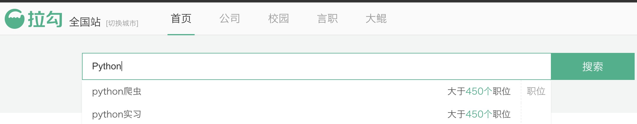
打开拉钩首页,https://www.lagou.com 进去选择全国站,搜索栏输入 Python,点击搜索
滚动到底部可以看到,页数只有30页:
点击下一页几次,发现页面并没有全部刷新,猜测是Ajax动态加载数据,
Chrome浏览器打开开发者工具进行抓包分析,勾XHR过滤,刷新网页

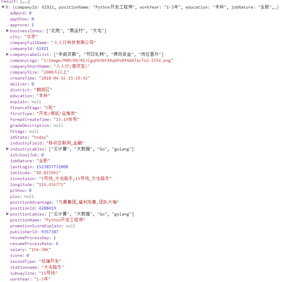
点击Preview选项卡查看具体的Json内容,发现第一个就是所需的数据

点开列表中的中的一个,这些就是可以采集的字段
知道拿哪里的数据,接下来就是模拟请求了,点击Header选项卡,
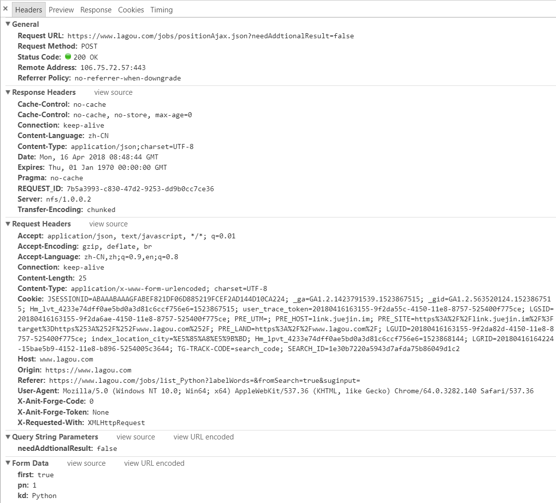
先是请求头,因为没登陆就可以访问了,Cookies就不用传了,其他都带上,
接着是Post提交的表单数据:
{ first:true,pn:2,kd:Python }
first是否第一次加载,pn参数是页码,kd是搜索关键词,爬取的时候只需修改页码,
其他两个参数不用动,接着编写一波代码爬取想要的数据,这里直接利用pandas库,
创建一个DataFrame对象,然后调用to_csv()函数把所有数据写入到csv文件中。、
这里还需判断是否为首页,是首页的话,设置下表头。
# Ajax加载urlajax_url = "https://www.lagou.com/jobs/positionAjax.json?"# url拼接参数request_params = {'needAddtionalResult': 'false'}# post提交参数form_data = {'first': 'false', 'pn': '1', 'kd': 'Python'}# 获得页数的正则page_pattern = re.compile('"totalCount":(\d*),', re.S)# csv表头csv_headers = ['公司id', '城市', '职位名称', '工作年限', '学历', '职位性质', '薪资','融资状态', '行业领域', '招聘岗位id', '公司优势', '公司规模','公司标签', '所在区域', '技能标签', '公司经度', '公司纬度', '公司全名']# 模拟请求头ajax_headers = {'Accept': 'application/json, text/javascript, */*; q=0.01','Accept-Encoding': 'gzip, deflate, br','Accept-Language': 'zh-CN,zh;q=0.9,en;q=0.8','Connection': 'keep-alive','Content-Type': 'application/x-www-form-urlencoded; charset=UTF-8','Host': 'www.lagou.com ','Origin': 'https://www.lagou.com ','User-Agent': 'Mozilla/5.0 (X11; Linux x86_64) AppleWebKit/537.36 (KHTML, like Gecko) Chrome/65.0.3325.146 Safari/537.36','X-Anit-Forge-Code': '0','X-Anit-Forge-Token': 'None','X-Requested-With': 'XMLHttpRequest','Referer': 'https://www.lagou.com/jobs/list_android?labelWords=&fromSearch=true&suginput='}# 获取每页招聘信息def fetch_data(page):fetch_url = ajax_url + urllib.parse.urlencode(request_params)global max_pagewhile True:try:form_data['pn'] = pageprint("抓取第:" + str(page) + "页!")# 随缘休息5-15s,避免因为访问过于频繁被封iptime.sleep(random.randint(5, 15))resp = requests.post(url=fetch_url, data=form_data, headers=ajax_headers)if resp.status_code == 200:if page == 1:max_page = int(int(page_pattern.search(resp.text).group(1)) / 15)print("总共有:" + str(max_page) + "页")data_json = resp.json()['content']['positionResult']['result']data_list = []for data in data_json:data_list.append((data['companyId'],data['city'],html.unescape(data['positionName']),data['workYear'],data['education'],data['jobNature'],data['salary'],data['financeStage'],data['industryField'],data['positionId'],html.unescape(data['positionAdvantage']),data['companySize'],data['companyLabelList'],data['district'],html.unescape(data['positionLables']),data['longitude'],data['latitude'],html.unescape(data['companyFullName'])))result = pd.DataFrame(data_list)if page == 1:result.to_csv(result_save_file, header=csv_headers, index=False, mode='a+')else:result.to_csv(result_save_file, header=False, index=False, mode='a+')return Noneexcept Exception as e:print(e)
注意:
在爬取文本信息的时候会遇到 和&这类HTML里的转义字符,需要调用html模块的
unescape()函数对此进行转义,对应函数escape(),比如上面爬取的文本有些如果不进行
转义的话,会出现写入结果错位的情况!
接着运行程序把数据写入到csv文件中

打开csv文件可以看到总共爬取到了1746条数据,数据有了,接下来就是准备开始
数据分析可视化了,在此之前我们先要简单了解下数据分析的两个常用库numpy与pandas。
1.2 numpy库基本了解
1.2.1 numpy简介
numpy库 科学计算的基础库,提供了一个多维数组对象(ndarray)和各种派生对象(如Masked arrays和矩阵),
以及各种加速数组操作的例程,包括数学、逻辑、图形变换、排序、选择、io、离散傅立叶变换、
基础线性代数、基础统计,随机模拟等等。
概念看上去很复杂,目前我们只需了解ndarray一些常用的基本函数的使用就够了,
如果有兴趣了解更多可移步到:https://docs.scipy.org/doc/numpy-dev/user/index.html
进行更深入的学习。
1.2.2 numpy安装
可以通过pip命令:pip install numpy
或者Anaconda库进行安装:conda install numpy
安装完后可以进入python测试下:import numpy,没有报错说明安装成功。
1.2.3 ndarray数组
ndarray是一个多维的数组对象,和Python自带的列表,元组等元素最大的区别
后者里元素的数据类型可以是不一样的,比如一个列表里可能放着整型,字符串,
而ndarray里的元素的数据类型必须是相同的!最简单的可以通过numpy提供的
array函数来生成一个ndarray数组,传入一个列表或者元组即可创建。接着演示
下如何生成ndarray的多种方法以及几个常用属性。
import numpy as npprint("1.生成一个一维数组:\n %s" % np.array([1, 2]))print("2.生成一个二维数组:\n %s" % np.array([[1, 2], [3, 4]]))print("3.生成一个元素初始值都为0的,4行3列矩阵:\n %s" % np.zeros((4, 3)))print("4.生成一个元素初始值都为1的,3行4列矩阵:\n %s" % np.ones((3, 4)))print("5.创建一个空数组,元素为随机值:\n %s" % np.empty([2, 3], dtype=int))a1 = np.arange(0, 30, 2)print("6.生成一个等间隔数字的数组:\n %s" % a1)a2 = a1.reshape(3, 5)print("7.转换数组的维度,比如把一维的转为3行5列的数组:\n %s" % a2)# ndarray常用属性print("8.a1的维度: %d \t a2的维度:%d" % (a1.ndim, a2.ndim))print("9.a1的行列数:%s \t a2的行列数:%s" % (a1.shape, a2.shape))print("10.a1的元素个数:%d \t a2的元素个数:%d" % (a1.size, a2.size))print("11.a1的元素数据类型:%s 数据类型大小:%s" % (a1.dtype, a1.itemsize))
运行结果
1.生成一个一维数组:[1 2]2.生成一个二维数组:[[1 2][3 4]]3.生成一个元素初始值都为0的,4行3列矩阵:[[0. 0. 0.][0. 0. 0.][0. 0. 0.][0. 0. 0.]]4.生成一个元素初始值都为1的,3行4列矩阵:[[1. 1. 1. 1.][1. 1. 1. 1.][1. 1. 1. 1.]]5.创建一个空数组,元素为随机值:[[ 0 1072693248 0][1072693248 0 1072693248]]6.生成一个等间隔数字的数组:[ 0 2 4 6 8 10 12 14 16 18 20 22 24 26 28]7.转换数组的维度,比如把一维的转为3行5列的数组,和元数组是内存共享的:[[ 0 2 4 6 8][10 12 14 16 18][20 22 24 26 28]]8.a1的维度: 1 a2的维度:29.a1的行列数:(15,) a2的行列数:(3, 5)10.a1的元素个数:15 a2的元素个数:1511.a1的元素数据类型:int32 数据类型大小:4
1.2.4 ndarray数组的常见操作
import numpy as np# 1.访问数组a1 = np.array([[1, 2, 3], [4, 5, 6], [7, 8, 9]])print("访问第一行: %s" % a1[0])a1[0] = 2 # 修改数组中元素的值print("访问第一列: %s" % a1[:, 0])print("访问前两行:\n {}".format(a1[:2]))print("访问前两列:\n {}".format(a1[:, :2]))print("访问第二行第三列:{}".format(a1[1][9]))# 2.通过take函数访问数组(axis参数代表轴),put函数快速修改元素值a2 = np.array([1, 2, 3, 4, 5])print("take函数访问第二个元素:%s" % a2.take(1))a3 = np.array([0, 2, 4])print("take函数参数列表索引元素:%s" % a2.take(a3))print("take函数访问某个轴的元素:%s" % a1.take(1, axis=1))a4 = np.array([6, 8, 9])a2.put([0, 2, 4], a4)print("put函数快速修改特定索引元素的值:%s" % a2)# 3.通过比较符访问元素print("通过比较符索引满足条件的元素:%s" % a1[a1 > 3])# 4.遍历数组print("一维数组遍历:")for i in a2:print(i, end=" ")print("\n二维数组遍历:")for i in a1:print(i, end=" ")print("\n还可以这样遍历:")for (i, j, k) in a1:print("%s - %s - %s" % (i, j, k))# 5.insert插入元素(参数依次为:数组,插入轴的标号,插入值,axis=0插入行,=1插入列)a5 = np.array([[1, 2, 3], [4, 5, 6], [7, 8, 9]])a5 = np.insert(a5, 0, [6, 6, 6], axis=0)print("insert函数插入元素到第一行:\n %s " % a5)# 6.delete删除元素(参数依次为数组,删除轴的标号,axis同上)a5 = np.delete(a5, 0, axis=1)print("delete函数删除第一列元素:\n %s" % a5)# 7.copy深拷贝一个数组,直接赋值是浅拷贝a6 = a5.copy()a7 = a5print("copy后的数组是否与原数组指向同一对象:%s" % (a6 is a5))print("赋值的数组是否与原数组指向同一对象:%s" % (a7 is a5))# 8.二维数组转一维数组,二维数组数组合并a8 = np.array([[1, 2, 3], [4, 5, 6], [7, 8, 9]])print("二维数组 => 一维数组:%s" % a8.flatten())a9 = np.array([[1, 2, 3], [4, 5, 6]])a10 = np.array([[7, 8], [9, 10]])print("两个二维数组合并 => 一个二维数组:\n{}".format(np.concatenate((a9, a10), axis=1)))# 9.数学计算(乘法是对应元素想成,叉乘用.dot()函数)a11 = np.array([[1, 2], [3, 4]])a12 = np.array([[5, 6], [7, 8]])print("数组相加:\n%s" % (a11 + a12))print("数组相减:\n%s" % (a11 - a12))print("数组相乘:\n%s" % (a11 * a12))print("数组相除:\n%s" % (a11 / a12))print("数组叉乘:\n%s" % (a11.dot(a12)))# 10.其他a12 = np.array([1, 2, 3, 4])print("newaxis增加维度:\n %s" % a12[:, np.newaxis])print("tile函数重复数组(重复列数,重复次数):\n %s" % np.tile(a12, [2, 2]))print("vstack函数按列堆叠:\n %s" % np.vstack([a12, a12]))print("hstack函数按行堆叠:\n %s" % np.hstack([a12, a12]))a13 = np.array([1, 4, 8, 2, 44, 77, -2, 1, 4])a13.sort()print("sort函数排序:\n %s" % a13)print("unique函数去重:\n {}".format(np.unique(a13)))
运行结果:
访问第一行: [1 2 3]访问第一列: [2 4 7]访问前两行:[[2 2 2][4 5 6]]访问前两列:[[2 2][4 5][7 8]]访问第二行第三列:6take函数访问第二个元素:2take函数参数列表索引元素:[1 3 5]take函数访问某个轴的元素:[2 5 8]put函数快速修改特定索引元素的值:[6 2 8 4 9]通过比较符索引满足条件的元素:[4 5 6 7 8 9]一维数组遍历:6 2 8 4 9二维数组遍历:[2 2 2] [4 5 6] [7 8 9]还可以这样遍历:2 - 2 - 24 - 5 - 67 - 8 - 9insert函数插入元素到第一行:[[6 6 6][1 2 3][4 5 6][7 8 9]]delete函数删除第一列元素:[[6 6][2 3][5 6][8 9]]copy后的数组是否与原数组指向同一对象:False赋值的数组是否与原数组指向同一对象:True二维数组 => 一维数组:[1 2 3 4 5 6 7 8 9]两个二维数组合并 => 一个二维数组:[[ 1 2 3 7 8][ 4 5 6 9 10]]数组相加:[[ 6 8][10 12]]数组相减:[[-4 -4][-4 -4]]数组相乘:[[ 5 12][21 32]]数组相除:[[ 0.2 0.33333333][ 0.42857143 0.5 ]]数组叉乘:[[19 22][43 50]]newaxis增加维度:[[1][10][3][11]]tile函数重复数组(重复列数,重复次数):[[1 2 3 4 1 2 3 4][1 2 3 4 1 2 3 4]]vstack函数按列堆叠:[[1 2 3 4][1 2 3 4]]hstack函数按行堆叠:[1 2 3 4 1 2 3 4]sort函数排序:[-2 1 1 2 4 4 8 44 77]unique函数去重:[-2 1 2 4 8 44 77]
1.3 pandas库基本了解
1.3.1 pandas简介
提供了快速便捷处理结构化数据的大量数据结构和函数,有两种数据
常见的数据结构,分别为:Series (一维的标签化数组对象)和 DataFrame (面向列的二维表结构)
同样是讲述库的基本使用,想深入了解pandas可移步到官网:
十分钟上手pandas:http://pandas.pydata.org/pandas-docs/stable/10min.html
更多内容:http://pandas.pydata.org/pandas-docs/stable/cookbook.html#cookbook
pandas库安装:pip install pandas
1.3.2 Series与DataFrame简介
Series是一维的标签化数组对象,和Python自带的列表类似,每个元素由索引与值构成,
数组中的值为相同的数据类型。
注意:np.nan用来标示空缺数据
Series
import pandas as pdimport numpy as nps1 = pd.Series([1, 2, 3, np.nan, 5])print("1.通过列表创建Series对象:\n%s" % s1)s2 = pd.Series([1, 2, 3, np.nan, 5], index=['a', 'b', 'c', 'd', 'e'])print("2.通过列表创建Series对象(自定义索引):\n%s" % s2)print("3.通过索引获取元素:%s" % s2['a'])print("4.获得索引:%s" % s2.index)print("5.获得值:%s" % s2.values)print("6.和列表一样值支持分片的:\n{}".format(s2[0:2]))s3 = pd.Series(pd.date_range('2018.3.17', periods=6))print("7.利用date_range生成日期列表:\n%s" % s3)
运行结果:
1.通过列表创建Series对象:0 1.01 2.02 3.03 NaN4 5.0dtype: float642.通过列表创建Series对象(自定义索引):a 1.0b 2.0c 3.0d NaNe 5.0dtype: float643.通过索引获取元素:1.04.获得索引:Index(['a', 'b', 'c', 'd', 'e'], dtype='object')5.获得值:[ 1. 2. 3. nan 5.]6.和列表一样值支持分片的:a 1.0b 2.0dtype: float647.利用date_range生成日期列表:0 2018-03-171 2018-03-182 2018-03-193 2018-03-204 2018-03-215 2018-03-22dtype: datetime64[ns]
DataFrame
面向列的二维表结构,类似于Excel表格,由行标签、列表索引与值三部分组成。
# 1.创建DataFrame对象dict1 = {'学生': ["小红", "小绿", "小蓝", "小黄", "小黑", "小灰"],'性别': ["女", "男", "女", "男", "男", "女"],'年龄': np.random.randint(low=10, high=15, size=6),}d1 = pd.DataFrame(dict1)print("1.用相等长度的列表组成的字典对象生成:\n %s" % d1)d2 = pd.DataFrame(np.random.randint(low=60, high=100, size=(6, 3)),index=["小红", "小绿", "小蓝", "小黄", "小黑", "小灰"],columns=["语文", "数学", "英语"])print("2.通过二维数组生成DataFrame: \n %s" % d2)# 2.数据查看print("3.head函数查看顶部多行(默认5行):\n%s" % d2.head(3))print("4.tail函数查看底部多行(默认5行):\n%s" % d2.tail(2))print("5.index查看所有索引:%s" % d2.index)print("6.columns查看所有行标签:%s" % d2.columns)print("7.values查看所有值:\n%s" % d2.values)# 3.数据排序print("8.按索引排序(axis=0行索引,=1列索引排序,ascending=False降序排列):\n%s"% (d2.sort_index(axis=0, ascending=False)))print("9.按值进行排序:\n%s" % d2.sort_values(by="语文", ascending=False))# 4.数据选择print("9.选择一列或多列:\n{} {} ".format(d2['语文'], d2[['数学', '英语']]))print("10.数据切片:\n{}".format(d2[0:1]))print("11.条件过滤(过滤语文分数高于90的数据):\n{}".format(d2[d2.语文 > 90]))print("12.loc函数行索引切片获得指定列数据:\n{}".format(d2.loc['小红':'小蓝', ['数学', '英语']]))print("13.iloc函数行号切片获得指定列数据:\n{}".format(d2.iloc[4:6, 1:2]))# 5.求和,最大/小值,平均值,分组print("14.语文总分:{}".format(d2['语文'].sum()))print("15.语文平均分:{}".format(d2['语文'].mean()))print("16.数学最高分:{}".format(d2['数学'].max()))print("17.英语最低分:{}".format(d2['英语'].min()))# 6.数据输入输出(可以把数据保存到csv或excel中,也可以读取文件)d1.to_csv('student_1.csv')d3 = pd.read_csv('student_1.csv')print("18.读取csv文件中的数据:\n{}".format(d3))d2.to_excel('student_2.xlsx', sheet_name="Sheet1")d4 = pd.read_excel('student_2.xlsx', sheet_name="Sheet1")print(("19.读取excel文件中的数据:\n{}".format(d4)))
运行结果:
1.用相等长度的列表组成的字典对象生成:学生 年龄 性别0 小红 10 女1 小绿 10 男2 小蓝 10 女3 小黄 12 男4 小黑 10 男5 小灰 11 女2.通过二维数组生成DataFrame:语文 数学 英语小红 96 96 77小绿 95 67 93小蓝 98 69 98小黄 65 81 94小黑 74 98 64小灰 96 72 963.head函数查看顶部多行(默认5行):语文 数学 英语小红 96 96 77小绿 95 67 93小蓝 98 69 984.tail函数查看底部多行(默认5行):语文 数学 英语小黑 74 98 64小灰 96 72 965.index查看所有索引:Index(['小红', '小绿', '小蓝', '小黄', '小黑', '小灰'], dtype='object')6.columns查看所有行标签:Index(['语文', '数学', '英语'], dtype='object')7.values查看所有值:[[96 96 77][95 67 93][98 69 98][65 81 94][74 98 64][96 72 96]]8.按索引排序(axis=0行索引,=1列索引排序,ascending=False降序排列):语文 数学 英语小黑 74 98 64小黄 65 81 94小蓝 98 69 98小绿 95 67 93小红 96 96 77小灰 96 72 969.按值进行排序:语文 数学 英语小蓝 98 69 98小红 96 96 77小灰 96 72 96小绿 95 67 93小黑 74 98 64小黄 65 81 949.选择一列或多列:小红 96小绿 95小蓝 98小黄 65小黑 74小灰 96Name: 语文, dtype: int64 数学 英语小红 96 77小绿 67 93小蓝 69 98小黄 81 94小黑 98 64小灰 72 9610.数据切片:语文 数学 英语小红 96 96 7711.条件过滤(过滤语文分数高于90的数据):语文 数学 英语小红 96 96 77小绿 95 67 93小蓝 98 69 98小灰 96 72 9612.loc函数行索引切片获得指定列数据:数学 英语小红 96 77小绿 67 93小蓝 69 9813.iloc函数行号切片获得指定列数据:数学小黑 98小灰 7214.语文总分:52415.语文平均分:87.3333333333333316.数学最高分:9817.英语最低分:6418.读取csv文件中的数据:Unnamed: 0 学生 年龄 性别0 0 小红 10 女1 1 小绿 10 男2 2 小蓝 10 女3 3 小黄 12 男4 4 小黑 10 男5 5 小灰 11 女19.读取excel文件中的数据:语文 数学 英语小红 96 96 77小绿 95 67 93小蓝 98 69 98小黄 65 81 94小黑 74 98 64小灰 96 72 96
1.4 matplotlib进行数据可视化
1.4.1 matplotlib简介
matplotlib是一个用于2D图表绘制的Python库。用法也很简单,可以
轻易地绘制出各种图表本节会用到几个常用的图形:直方图,饼图,条形图;
官方文档中还有各种各样的图以及Demo示例:

有兴趣可移步到:
Matplotlib入门教程:https://pythonprogramming.net/matplotlib-intro-tutorial/
Matplotlib绘制各种图形Demo示例:https://matplotlib.org/gallery.html#lines_bars_and_markers
推荐通过pip命令行进行安装:pip install matplotlib
1.4.2 matplotlib中文乱码问题
使用matplotlib进行图表绘制,第一个遇到的问题就是中文乱码问题,如图
解决方法如下:
1.编写如下代码获得matplotlib库配置相关的路径:
import matplotlibprint(matplotlib.matplotlib_fname())
接着会获得一个对应的路径,比如我的电脑是:
/usr/local/lib/python3.4/dist-packages/matplotlib/mpl-data/matplotlibrc
2.下载一个文中的ttf字体文件(任意),然后把文件拷贝到这个路径下,双击安装;
3.接着修改matplotlibrc配置文件,找到如下三行,去掉注释,进行修改:
199行:font.family : sans-serif210行:font.serif : 中文字体名称, DejaVu Serif, Bitstream330行:axes.unicode_minus : False
4.删除.cache/matplotlib缓存文件,重新运行即可。
1.4.3 matplotlib绘制显示不全
如图,在绘制的时候可能会出现显示不全的情况,需要进行设置,
顺道介绍下下面7个菜单按钮的,依次是:
重置回主视图,上一步视图,下一步视图,拖拽页面,
局部放大,设置,保存成图片
点击设置,会出现如图所示对话框:
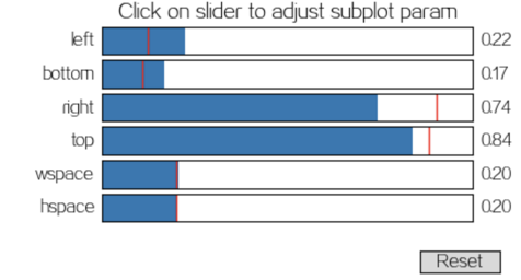
拖拉调整下,直到差不多显示完全
记录下这些参数,在绘制图形之前,需要代码设置下:
plt.subplots_adjust(left=0.22, right=0.74, wspace=0.20, hspace=0.20,bottom=0.17, top=0.84)
1.4.4 matplotlib生成图表并进行分析
先调用pd.read_csv()函数读取一开始爬取数据存放的csv文件,接着开始针对不同的列进行数据分析,
1.公司规模(饼图)
plt.figure(1)data['公司规模'].value_counts().plot(kind='pie', autopct='%1.1f%%',explode=np.linspace(0, 0.5, 6))plt.subplots_adjust(left=0.22, right=0.74, wspace=0.20, hspace=0.20,bottom=0.17, top=0.84)plt.savefig(pic_save_path + 'result_1.jpg')plt.close(1)
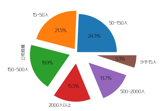
招Python的公司规模都比较平均,中小型公司(15-500人)占比达81% 。
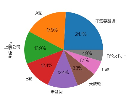
2.公司融资状态(饼图)
plt.figure(2)data['融资状态'].value_counts().plot(kind='pie', autopct='%1.1f%%')plt.subplots_adjust(left=0.22, right=0.74, wspace=0.20, hspace=0.20,bottom=0.17, top=0.84)plt.savefig(pic_save_path + 'result_2.jpg')plt.close(2)
3.公司城市分布(饼图)
plt.figure(3)data['城市'].value_counts().plot(kind='pie', autopct='%1.1f%%')plt.subplots_adjust(left=0.31, right=0.74, wspace=0.20, hspace=0.20,bottom=0.26, top=0.84)plt.savefig(pic_save_path + 'result_3.jpg')plt.close(3)
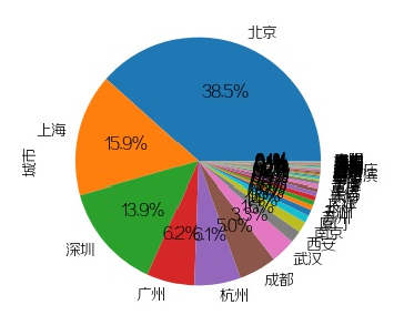
招Python开发排名前几的城市依次为:
北京,上海,深圳,广州,杭州,成都,武汉,西安,南京,厦门
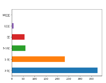
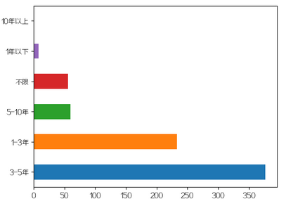
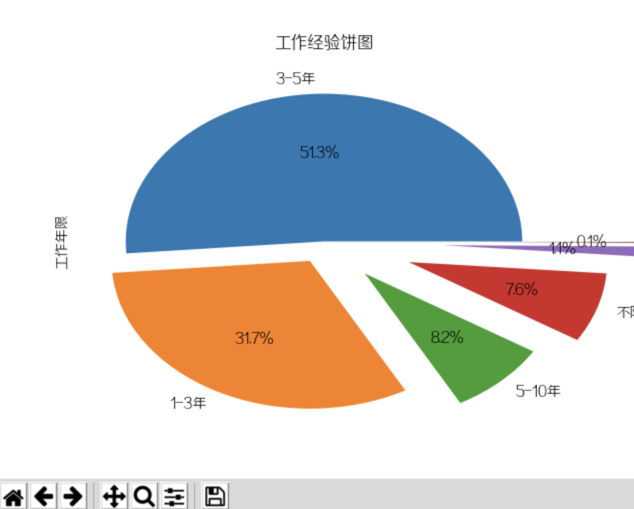
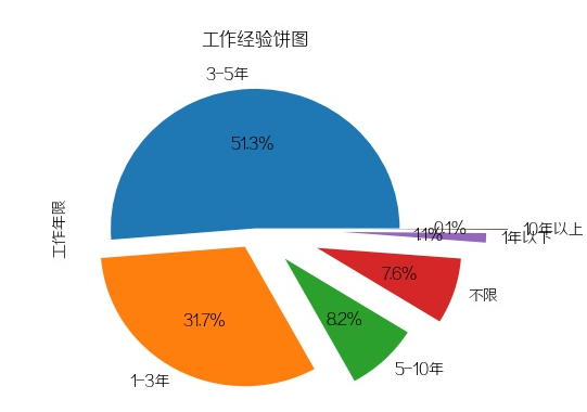
4.要求工作经验(直方图+饼图)
plt.figure(4)data['工作年限'].value_counts().plot(kind='barh', rot=0)plt.title("工作经验直方图")plt.xlabel("年限/年")plt.ylabel("公司/个")plt.savefig(pic_save_path + 'result_4.jpg')plt.close(4)# 饼图plt.figure(5)data['工作年限'].value_counts().plot(kind='pie', autopct='%1.1f%%', explode=np.linspace(0, 0.75, 6))plt.title("工作经验饼图")plt.subplots_adjust(left=0.22, right=0.74, wspace=0.20, hspace=0.20,bottom=0.17, top=0.84)plt.savefig(pic_save_path + 'result_5.jpg')plt.close(5)


工作1-3年与3-5年的Python工程师依旧比较抢手。
5.学历要求(饼图)
plt.figure(6)data['学历'].value_counts().plot(kind='pie', autopct='%1.1f%%', explode=(0, 0.1, 0.2,0.3))plt.title("学历饼图")plt.subplots_adjust(left=0.22, right=0.74, wspace=0.20, hspace=0.20,bottom=0.17, top=0.84)plt.savefig(pic_save_path + 'result_6.jpg')plt.close(6)
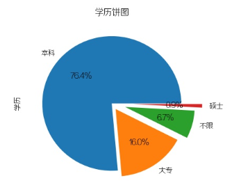
接近七成半的公司需要本科学历以上!
6.薪资(条形图)
plt.figure(7)salary = data['薪资'].str.split('-').str.get(0).str.replace('k|K|以上', "").value_counts()salary_index = list(salary.index)salary_index.sort(key=lambda x: int(x))final_salary = salary.reindex(salary_index)plt.title("薪资条形图")final_salary.plot(kind='bar', rot=0)plt.xlabel("薪资/K")plt.ylabel("公司/个")plt.savefig(pic_save_path + 'result_7.jpg')plt.close(7)

结合工作经验饼图分析,猜测1-3年初级Python开发者的薪资范围为:8-10k,
而3-5年的中级Python开发者的薪资范围为: 10-15k。
1.5 wordcloud绘制词云
1.5.1 wordcloud简介
上面这类有具体数值的数据,可以通过图表形式来表现,而除了这类数据
外还有一种,比如公司标签这一类数据
我们可以进行词频统计,即每个词语出现的次数,接着按照比例生成词云。
而生成词云可以利用wordcloud这个库,这里同样只介绍基础用法,更多
可移步到下述网址:
Github仓库:https://github.com/amueller/word_cloud
官方博客:https://amueller.github.io/word_cloud/
推荐通过pip命令行进行安装:pip install wordcloud
1.5.2 WordCloud构造函数与常用方法
构造函数
def __init__(self, font_path=None, width=400, height=200, margin=2,ranks_only=None, prefer_horizontal=.9, mask=None, scale=1,color_func=None, max_words=200, min_font_size=4,stopwords=None, random_state=None, background_color='black',max_font_size=None, font_step=1, mode="RGB",relative_scaling=.5, regexp=None, collocations=True,colormap=None, normalize_plurals=True):
参数详解:
- font_path:字体路径,就是绘制词云用的字体,比如monaco.ttf
- width:输出的画布宽度,默认400像素
- height:输出的画布宽度,默认200像素
- margin:画布偏移,默认2像素
- prefer_horizontal : 词语水平方向排版出现的频率,默认0.9,垂直方向出现概率0.1
- mask:如果参数为空,则使用二维遮罩绘制词云。如果 mask 非空,设置的宽高值将
被忽略,遮罩形状被 mask,除全白(#FFFFFF)的部分将不会绘制,其余部分会用于绘制词云。
如:bg_pic = imread('读取一张图片.png'),背景图片的画布一定要设置为白色(#FFFFFF),
然后显示的形状为不是白色的其他颜色。可以用ps工具将自己要显示的形状复制到一个纯白色
的画布上再保存,就ok了。 - scale:按照比例进行放大画布,如设置为1.5,则长和宽都是原来画布的1.5倍
- color_func:生成新颜色的函数,如果为空,则使用 self.color_func
- max_words:显示的词的最大个数
- min_font_size:显示的最小字体大小
- stopwords:需要屏蔽的词(字符串集合),为空使用内置STOPWORDS
- random_state:如果给出了一个随机对象,用作生成一个随机数
- background_color:背景颜色,默认为黑色
- max_font_size:显示的最大的字体大小
- font_step:字体步长,如果步长大于1,会加快运算但是可能导致结果出现较大的误差
- mode:当参数为"RGBA",并且background_color不为空时,背景为透明。默认RGB
- relative_scaling:词频和字体大小的关联性,默认5
- regexp:使用正则表达式分隔输入的文本
- collocations:是否包括两个词的搭配
- colormap:给每个单词随机分配颜色,若指定color_func,则忽略该方法
- normalize_plurals:是否删除尾随的词语
常用的几个方法:
- fit_words(frequencies):根据词频生成词云
- generate(text):根据文本生成词云
- generate_from_frequencies(frequencies[, ...]):根据词频生成词云
- generate_from_text(text):根据文本生成词云
- process_text(text):将长文本分词并去除屏蔽词
(此处指英语,中文分词还是需要自己用别的库先行实现,使用上面的 fit_words(frequencies) ) - recolor([random_state, color_func, colormap]) :
对现有输出重新着色。重新上色会比重新生成整个词云快很多。 - to_array():转化为 numpy array
- to_file(filename):输出到文件
1.5.3 WordCloud绘制词云
看上面的字段和函数那么多,感觉wordcloud很难用,其实并不难,笔者
写个最简单的绘制方法,自己参照着上面按需进行扩展就好。
# 生成词云文件(参数为词云字符串与文件名,default_font是一个ttf的字体文件)def make_wc(content, file_name):wc = WordCloud(font_path=default_font, background_color='white', margin=2,max_font_size=250,width=2000, height=2000,min_font_size=30, max_words=1000)wc.generate_from_frequencies(content)wc.to_file(file_name)
接着再需要绘制词云的地方调用该函数即可,比如这里生成行业领域词云:
industry_field_list = []for industry_field in data['行业领域']:for field in str(industry_field).strip().replace(" ", ",").replace("、", ",").split(','):industry_field_list.append(field)counter = dict(Counter(industry_field_list))counter.pop('')make_wc(counter, pic_save_path + "wc_1.jpg")

招Python开发的公司大部分是移动互联网的,其次是数据服务。
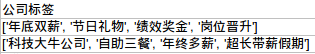
2.公司标签
tags_list = []for tags in data['公司标签']:for tag in tags.strip().replace("[", "").replace("]", "")\.replace("'", "").split(','):tags_list.append(tag)counter = dict(Counter(tags_list))counter.pop('')make_wc(counter, pic_save_path + "wc_2.jpg")

3.公司优势
for advantage_field in data['公司优势']:for field in advantage_field.strip().replace(" ", ",")\.replace("、", ",").replace(",", ",").replace("+", ",").split(','):industry_field_list.append(field)counter = dict(Counter(industry_field_list))counter.pop('')counter.pop('移动互联网')make_wc(counter, pic_save_path + "wc_3.jpg")

4.技能标签
skill_list = []for skills in data['技能标签']:for skill in skills.strip().replace("[", "").replace("]", "").replace("'", "").split(','):skill_list.append(skill)counter = dict(Counter(skill_list))counter.pop('')make_wc(counter, pic_save_path + "wc_4.jpg")

1.6 小结
有了这些图片后就可以自行做数据报告了,
