计算物理第十二次作业Problem5.1

---

摘要

在前面的课程中我们已经学习了微分方程的求解方式，而这一节我们将通过Gauss-Sideal Method来求解拉普拉斯方程。

背景介绍

已知电场的Laplace's equation为：

$$\frac{\partial^2 V}{\partial x^2}+\frac{\partial^2 V}{\partial y^2}+\frac{\partial^2 V}{\partial z^2}=0$$
微分可得： $$\begin{eqnarray*} \frac{\partial V}{\partial x}&\approx&\frac{V(i+1,j,k)-V(i,j,k)}{\Delta x}\\ \frac{\partial V}{\partial x}&\approx&\frac{V(i,j,k)-V(i-1,j,k)}{\Delta x}\\ \frac{\partial V}{\partial x}&\approx&\frac{V(i+1,j,k)-V(i-1,j,k)}{2\Delta x}\\ \frac{\partial^2 V}{\partial x^2}&=&\frac{1}{\Delta x}[\frac{\partial V}{\partial x}(i+\frac12)-\frac{\partial V}{\partial x}(i-\frac12)]\\ &\approx&\frac{V(i+1,j,k)+V(i-1,j,k)-2V(i,j,k)}{(\Delta x)^2} \end{eqnarray*}$$
由5.1可知，Gauss-Sideal Method有：
$$V_{new}(i,j)=\frac{1}{4}[V_{old}(i+1,j)+V_{new}(i-1,j)+V_{old}(i,j+1)+V_{new}(i,j-1)]$$

正文

关于电势的程序为：

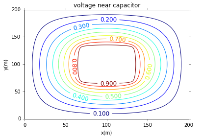
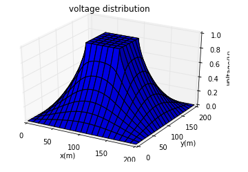
from __future__ import division
import matplotlib
import numpy as np
import matplotlib.cm as cm
import matplotlib.mlab as mlab
import matplotlib.pyplot as plt
from mpl_toolkits.mplot3d import Axes3D
# initialize the grid
grid = []
for i in range(201):    
    row_i = []
    for j in range(201):
        if i == 0 or i == 200 or j == 0 or j == 200:
            voltage = 0
        elif 70<=i<=130 and j == 70:
            voltage = 1
        elif 70<=i<=130 and j == 130:
            voltage = 1
        elif 70<=j<=130 and i == 70:
            voltage = 1
        elif 70<=j<=130 and i == 130:
            voltage = 1
        else:
            voltage = 0
        row_i.append(voltage)
    grid.append(row_i)
# define the update_V function (Gauss-Seidel method)
def update_V(grid):
    delta_V = 0
    for i in range(201):    
        for j in range(201):
            if i == 0 or i == 200 or j == 0 or j == 200:
                pass
            elif 70<=i<=130 and j == 70:
                pass
            elif 70<=i<=130 and j == 130:
                pass
            elif 70<=j<=130 and i == 70:
                pass
            elif 70<=j<=130 and i == 130:
                pass
            else:
                voltage_new = (grid[i+1][j]+grid[i-1][j]+grid[i][j+1]+grid[i][j-1])/4
                voltage_old = grid[i][j]
                delta_V += abs(voltage_new - voltage_old)
                grid[i][j] = voltage_new
    return grid, delta_V
# define the Laplace_calculate function
def Laplace_calculate(grid):
    epsilon = 10**(-5)*200**2
    grid_init = grid
    delta_V = 0
    N_iter = 0
    while delta_V >= epsilon or N_iter <= 10:
        grid_impr, delta_V = update_V(grid_init)
        grid_new, delta_V = update_V(grid_impr)
        grid_init = grid_new
        N_iter += 1
    return grid_new
matplotlib.rcParams['xtick.direction'] = 'out'
matplotlib.rcParams['ytick.direction'] = 'out'
x = np.linspace(0,200,201)
y = np.linspace(0,200,201)
X, Y = np.meshgrid(x, y)
Z = Laplace_calculate(grid)
plt.figure()
CS = plt.contour(X,Y,Z,10)
plt.clabel(CS, inline=1, fontsize=12)
plt.title('voltage near capacitor')
plt.xlabel('x(m)')
plt.ylabel('y(m)')
fig = plt.figure()
ax = fig.add_subplot(111, projection='3d')
ax.plot_surface(X, Y, Z)
ax.set_xlabel('x(m)')
ax.set_ylabel('y(m)')
ax.set_zlabel('voltage(V)')
ax.set_title('voltage distribution')
plt.show()

运行结果为：


关于电场的程序为：

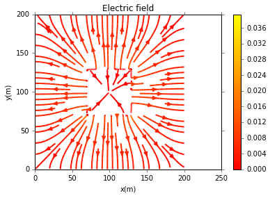
from __future__ import division
import matplotlib
import numpy as np
import matplotlib.cm as cm
import matplotlib.mlab as mlab
import matplotlib.pyplot as plt
from mpl_toolkits.mplot3d import Axes3D
from copy import deepcopy
# initialize the grid
grid = []
for i in range(201):    
    row_i = []
    for j in range(201):
        if i == 0 or i == 200 or j == 0 or j == 200:
            voltage = 0
        elif 70<=i<=130 and j == 70:
            voltage = 1
        elif 70<=i<=130 and j == 130:
            voltage = 1
        elif 70<=j<=130 and i == 70:
            voltage = 1
        elif 70<=j<=130 and i == 130:
            voltage = 1
        else:
            voltage = 0
        row_i.append(voltage)
    grid.append(row_i)
# define the update_V function (Gauss-Seidel method)
def update_V(grid):
    delta_V = 0
    for i in range(201):    
        for j in range(201):
            if i == 0 or i == 200 or j == 0 or j == 200:
                pass
            elif 70<=i<=130 and j == 70:
                pass
            elif 70<=i<=130 and j == 130:
                pass
            elif 70<=j<=130 and i == 70:
                pass
            elif 70<=j<=130 and i == 130:
                pass
            else:
                voltage_new = (grid[i+1][j]+grid[i-1][j]+grid[i][j+1]+grid[i][j-1])/4
                voltage_old = grid[i][j]
                delta_V += abs(voltage_new - voltage_old)
                grid[i][j] = voltage_new
    return grid, delta_V
# define the Laplace_calculate function
def Laplace_calculate(grid):
    epsilon = 10**(-5)*200**2
    grid_init = grid
    delta_V = 0
    N_iter = 0
    while delta_V >= epsilon or N_iter <= 10:
        grid_impr, delta_V = update_V(grid_init)
        grid_new, delta_V = update_V(grid_impr)
        grid_init = grid_new
        N_iter += 1
    return grid_new
x = np.linspace(0,200,201)
y = np.linspace(0,200,201)
X, Y = np.meshgrid(x, y)
Z = Laplace_calculate(grid)
Ex = deepcopy(Z)
Ey = deepcopy(Z)
E = deepcopy(Z)
for i in range(201):
    for j in range(201):
        if i == 0 or i == 200 or j == 0 or j == 200:
            Ex[i][j] = 0
            Ey[i][j] = 0
        else:
            Ex_value = -(Z[i+1][j] - Z[i][j])/2
            Ey_value = -(Z[i][j+1] - Z[i][j])/2
            Ex[i][j] = Ex_value
            Ey[i][j] = Ey_value
for i in range(201):
    for j in range(201):
        E_value = np.sqrt(Ex[i][j]**2 + Ey[i][j]**2)
        E[i][j] = E_value
fig0, ax0 = plt.subplots()
strm = ax0.streamplot(X, Y, np.array(Ey), np.array(Ex), color=np.array(E), linewidth=2, cmap=plt.cm.autumn)
fig0.colorbar(strm.lines)
ax0.set_xlabel('x(m)')
ax0.set_ylabel('y(m)')
ax0.set_title('Electric field')
plt.show()

运行结果为：

结论

对于prism geometry，势能和电场便如程序运行结果所示。

致谢

感谢贺一珺同学的程序。