计算物理第八次作业

计算物理

摘要

经过上次的学习和作业练习，我们更深刻地理解了混沌运动的图像及其性质，在此基础上，我们将进一步探究混沌现象的性质，同时尝试使用Vpython对程序结果进行表达。本次作业主要对于习题3.18， 3.19， 3.20， 3.21的相关习题进行探究和解答，并借此练习Vpython的使用。

背景介绍

经过我们上次的学习，我们发现混沌现象与$F_D$有关，但当我们连续改变$F_D$值时，又会发现新的现象。同时，就3D动画演示来说，对于我们更形象理解物体的运动有极大的帮助，本次的新平台Vpython便是一个非常好的工具，因此对它的掌握也是十分必要的。

正文

1. Problem 3.18

1.1
首先我们先回顾上周的程序，即做出figure 3.9，此处我们对程序略作修改，将精度改为0.01，步长提高到50000步，
尽管运行时需要时间，但图像质量较好，如下：

import pylab as pl
import math
class Simple_Pendulum :
    def __init__(self,i=0,initial_theta=0.2,time_step=0.04,total_time=50000,length=9.8,\
                 g=9.8, initial_omega=0,q=0.5,Fd=1.2,omegaD=0.66667):
        self.theta=[initial_theta]
        self.theta0=[initial_theta]
        self.t=[0]
        self.omega=[initial_omega]
        self.dt=time_step
        self.time=total_time
        self.g=g 
        self.l=length
        self.q=q
        self.Fd=Fd
        self.omegaD=omegaD
        self.a=[0]
        self.b=[0]
    def run(self):
        _time=0
        while(_time<self.time):
            self.omega.append(self.omega[-1]-((self.g/self.l)*math.sin(self.theta[-1])+\
                 self.q*self.omega[-1]-self.Fd*math.sin(self.omegaD*self.t[-1]))*self.dt)            
            self.theta.append(self.theta[-1]+self.omega[-1]*self.dt)
            self.t.append(_time)            
            _time += self.dt
            if(self.theta[-1]>=math.pi):
                self.theta[-1]=self.theta[-1]-2*math.pi
            if(self.theta[-1]<=-math.pi):
                self.theta[-1]=self.theta[-1]+2*math.pi
            if((self.t[-1])%(2*math.pi/self.omegaD)<0.01 ):
                self.a.append(self.omega[-1])
                self.b.append(self.theta[-1])
    def show_results(self):
        pl.plot(self.b,self.a,'.',label='$F_{D}$=1.2')
        pl.xlabel('$\\theta$(rad)')
        pl.ylabel('$\omega$(rad)')
        pl.legend()
        pl.title('$\omega$ versus $\\theta$ ' )
        pl.show()        
a = Simple_Pendulum()
a.run()
a.show_results()  

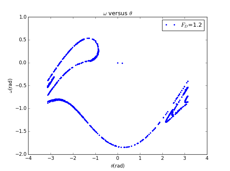
当然，我们可以改变$F_D$的取值以得到不同情况下的图像，如下：

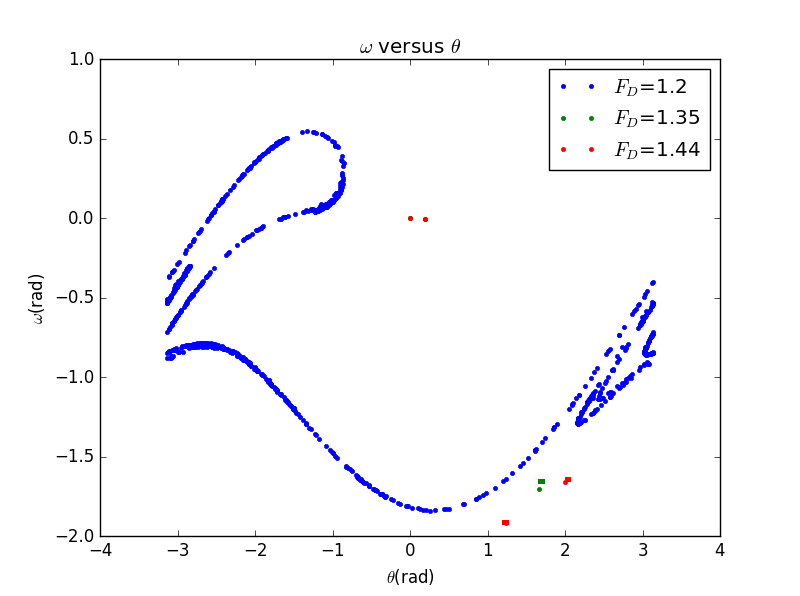
显然，混沌效应只在特殊的值附近出现，在图中即$F_D=1.2$时

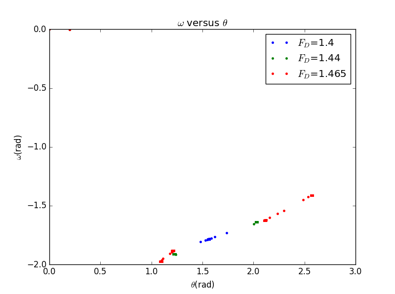
1.2
然后我们进一步改变$F_D$的取值,分别取为1.4，1.44，1.465，同时依据Figure 3.10修改其他参数，即：time step(dt)=0.01，q=1/2，l=g=9.8，$\Omega_D=2/3$
则图像如下：

2. Problem 3.20

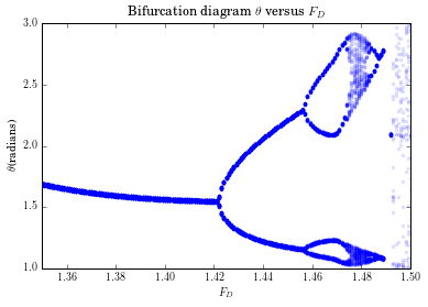
这里我们将试图做出类似Figure 3.11的图像，即$\theta$与$F_D$的关系图，其中$F_D$取值范围为1.35-1.5

2.1
我们利用上次课的结论，做出$\theta$和时间的图像，当我们取$F_D=1.35$时获得如下图像：

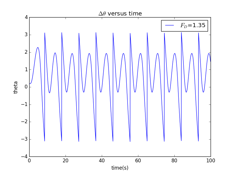
随着我们增加$F_D$的值，令其为1.44，图像变为：

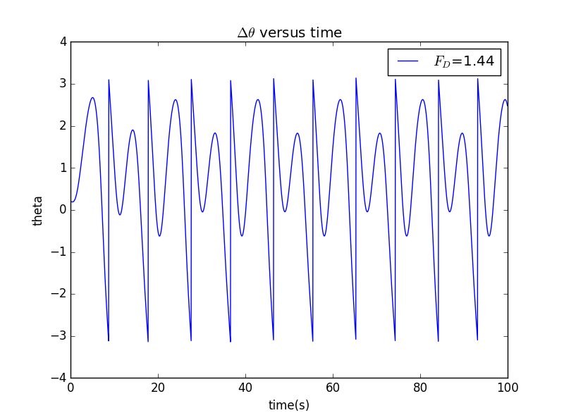
发现此时相当于周期变为原来的两倍，我们继续增加$F_D$,令其为1.465，图像如下：

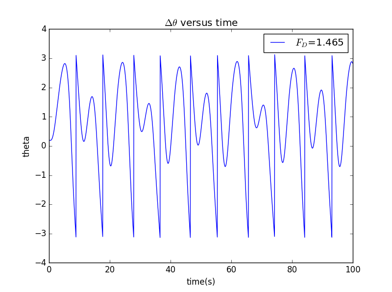
此时的函数图像周期显然为初始的四倍，这种现象即为“周期加倍”（Period doubling）
2.2
我们通过bifurcation diagram方法进行分析发现，在300个驱动力周期之后，$\theta$将不受初始值影响，即此时应为周期振动，因此当我们取300周期后，且符合$t=2n\pi/\Omega_D$时，每相空间内每周期会打出一个点，且该点应为$F_D$的函数。这样我们便可以画出$\theta$ 关于$F_D$的图像。
我们修改的主体程序如下：

import pylab as pl
import math
class Simple_Pendulum :
    def __init__(self,i=0,initial_theta=0.2,time_step=0.01,total_time=900*math.pi+10,length=9.8,\
                 g=9.8, initial_omega=0,q=0.5,Fd=1.35,omegaD=0.666667):
        self.theta=[initial_theta]
        self.theta0=[initial_theta]
        self.t=[0]
        self.omega=[initial_omega]
        self.dt=time_step
        self.time=total_time
        self.g=g 
        self.l=length
        self.q=q
        self.Fd=[Fd]
        self.F_d=[Fd]
        self.omegaD=omegaD
        self.a=[0]
        self.b=[0]
        self.a0=[0]
        self.b0=[0]
        self.b1=[0]
    def run(self):
        _time=0
        self.Fd=[1.35]        
        while(1):
           while(_time<self.time):
                self.omega.append(self.omega[-1]-((self.g/self.l)*math.sin(self.theta[-1])+\
                     self.q*self.omega[-1]-self.Fd[-1]*math.sin(self.omegaD*self.t[-1]))*self.dt)            
                self.theta.append(self.theta[-1]+self.omega[-1]*self.dt)
                self.t.append(_time)            
                _time += self.dt
                if(self.theta[-1]>=math.pi):
                    self.theta[-1]=self.theta[-1]-2*math.pi
                if(self.theta[-1]<=-math.pi):
                    self.theta[-1]=self.theta[-1]+2*math.pi
                if(self.t[-1]>(900*math.pi)):
                    self.a0.append(self.omega[-1])
                    self.b0.append(self.theta[-1])
                if((self.t[-1])%(3*math.pi)<0.01 ):
                    self.a.append(self.a0[-1])
                    self.b.append(self.b0[-1])
           self.b1.append(self.b[-1])
           self.Fd.append(self.Fd[-1]+0.01)
           if(self.Fd[-1]>1.5):
               break
    def show_results(self):
        pl.plot(self.Fd,self.b1,'.')
        pl.xlabel('$F_{D}$')
        pl.ylabel('$\\theta$(rad)')
        pl.legend()
        pl.title('$\omega$ versus $\\theta$ ' )
        pl.show()        
a = Simple_Pendulum()
a.run()
a.show_results()  

做图如下：

3.使用Vpython模拟摆的运动

对于混沌效应，我们可以进一步使用Vpython工具，将相空间内展示的东西通过动画做出，这里，我们以程序中自带例子来看：

scene.title = 'Double Pendulum'
scene.height = scene.width = 800
g = 9.8
M1 = 2.0
M2 = 1.0
L1 = 0.5 # physical length of upper assembly; distance between axles
L2 = 1.0 # physical length of lower bar
I1 = M1*L1**2/12 # moment of inertia of upper assembly
I2 = M2*L2**2/12 # moment of inertia of lower bar
d = 0.05 # thickness of each bar
gap = 2*d # distance between two parts of upper, U-shaped assembly
L1display = L1+d # show upper assembly a bit longer than physical, to overlap axle
L2display = L2+d/2 # show lower bar a bit longer than physical, to overlap axle
hpedestal = 1.3*(L1+L2) # height of pedestal
wpedestal = 0.1 # width of pedestal
tbase = 0.05 # thickness of base
wbase = 8*gap # width of base
offset = 2*gap # from center of pedestal to center of U-shaped upper assembly
top = vector(0,0,0) # top of inner bar of U-shaped upper assembly
scene.center = top-vector(0,(L1+L2)/2.,0)
theta1 = 2.1 # initial upper angle (from vertical)
theta2 = 2.4 # initial lower angle (from vertical)
theta1dot = 0 # initial rate of change of theta1
theta2dot = 0 # initial rate of change of theta2
pedestal = box(pos=top-vector(0,hpedestal/2.,offset),
                 height=1.1*hpedestal, length=wpedestal, width=wpedestal,
                 color=(0.4,0.4,0.5))
base = box(pos=top-vector(0,hpedestal+tbase/2.,offset),
                 height=tbase, length=wbase, width=wbase,
                 color=pedestal.color)
axle = cylinder(pos=top-vector(0,0,gap/2.-d/4.), axis=(0,0,-offset), radius=d/4., color=color.yellow)
frame1 = frame(pos=top)
bar1 = box(frame=frame1, pos=(L1display/2.-d/2.,0,-(gap+d)/2.), size=(L1display,d,d), color=color.red)
bar1b = box(frame=frame1, pos=(L1display/2.-d/2.,0,(gap+d)/2.), size=(L1display,d,d), color=color.red)
axle1 = cylinder(frame=frame1, pos=(L1,0,-(gap+d)/2.), axis=(0,0,gap+d),
                 radius=axle.radius, color=axle.color)
frame1.axis = (0,-1,0)
frame2 = frame(pos=frame1.axis*L1)
bar2 = box(frame=frame2, pos=(L2display/2.-d/2.,0,0), size=(L2display,d,d), color=color.green)
frame2.axis = (0,-1,0)
frame1.rotate(axis=(0,0,1), angle=theta1)
frame2.rotate(axis=(0,0,1), angle=theta2)
frame2.pos = top+frame1.axis*L1
dt = 0.00005 # energy constancy check fails for dt > 0.0003
t = 0.
C11 = (0.25*M1+M2)*L1**2+I1
C22 = 0.25*M2*L2**2+I2
#### For energy check:
##gdisplay(x=800)
##gK = gcurve(color=color.yellow)
##gU = gcurve(color=color.cyan)
##gE = gcurve(color=color.red)
while True:
    rate(1/dt)
    # Calculate accelerations of the Lagrangian coordinates:
    C12 = C21 = 0.5*M2*L1*L2*cos(theta1-theta2)
    Cdet = C11*C22-C12*C21
    a = .5*M2*L1*L2*sin(theta1-theta2)
    A = -(.5*M1+M2)*g*L1*sin(theta1)-a*theta2dot**2
    B = -.5*M2*g*L2*sin(theta2)+a*theta1dot**2
    atheta1 = (C22*A-C12*B)/Cdet
    atheta2 = (-C21*A+C11*B)/Cdet
    # Update velocities of the Lagrangian coordinates:
    theta1dot += atheta1*dt
    theta2dot += atheta2*dt
    # Update Lagrangian coordinates:
    dtheta1 = theta1dot*dt
    dtheta2 = theta2dot*dt
    theta1 += dtheta1
    theta2 += dtheta2
    frame1.rotate(axis=(0,0,1), angle=dtheta1)
    frame2.pos = top+frame1.axis*L1
    frame2.rotate(axis=(0,0,1), angle=dtheta2)
    t = t+dt
## Energy check:
##    K = .5*((.25*M1+M2)*L1**2+I1)*theta1dot**2+.5*(.25*M2*L2**2+I2)*theta2dot**2+\
##        .5*M2*L1*L2*cos(theta1-theta2)*theta1dot*theta2dot
##    U = -(.5*M1+M2)*g*L1*cos(theta1)-.5*M2*g*L2*cos(theta2)
##    gK.plot(pos=(t,K))
##    gU.plot(pos=(t,U))
##    gE.plot(pos=(t,K+U))

该程序即展示了双摆的运动动画，其效果如下

我们可以由此程序为基础进行进一步改进，但由于个人原因并未完全掌握Vpython，后续会对此次作业进行补充

结论

1.对于习题3.18

2.对于习题3.20

致谢

与张梓桐同学讨论了Problem 3.20的一些细节
与冉峰同学交流了一些思路和方法
Vpython自带程序