张梓桐 第五次计算物理

1 Problem

With the base of Page 34 on textbook.I fantastically consider the track of an cannon shell with air resistance,density of air(both aidabatic and isothermal approximation),and the variation of gravity via altitude.

2 Abstract

In this passage,we are going to talk about the different factors that may have effects on the movment of a cannon shell by Euler method.

3 Background Introduction

Acquiring from the previous knowledge of the Euler applied into the Computational Physics,we now can conclude more relastic factors into the movement of a cannon shell.
Now I still want to stress the importance of Euler method in the projectile movement:

$$\begin{eqnarray*} \frac{d^{2}x}{dt^{2}}=0\quad \frac{d^{2}y}{dt^{2}}=g \end{eqnarray*}$$
It seems impossible to use the Euler method as there's a order two differentiation.But as we substitute the variables,the solution appears above the fog clearly:
$$\begin{eqnarray*} \frac{dx}{dt}=v_{x}\quad \frac{dv_{x}}{dt}=0 \end{eqnarray*}$$
$$\begin{eqnarray*} \frac{dy}{dt}=v_{y}\quad \frac{dv_{y}}{dt}=-g \end{eqnarray*}$$
Here we change this into finite difference form:
$$\begin{eqnarray*} x_{i+1}=x_{i}+v_{x,i}\Delta t\quad v_{x,i+1}=v_{x,i} \end{eqnarray*}$$
$$\begin{eqnarray*} y_{i+1}=y_{i}+v_{y,i}\Delta t\quad v_{y,i+1}=v_{y,i}-g\Delta t \end{eqnarray*}$$
Now we already have the basic knowldege of projectile movement,next we want to focus on the different factors that affect the solution:

3.1 Resistance:

There will add one extra term in each equation of velocity:

$$\begin{eqnarray*} v_{x,i+1}=v_{x,i}-\frac{B_{2}vv_{x,i}}{m}\Delta t \end{eqnarray*}$$
$$\begin{eqnarray*} v_{y,i+1}=v_{y,i}-\frac{B_{1}vv_{y,i}}{m}\Delta t-g\Delta t \end{eqnarray*}$$

3.2 Effects of altitude on air density:

3.2.1 The isothermal situation:

$$\begin{eqnarray*} \rho(y)=\rho(0)e^{-\frac{y}{y_{0}}} \end{eqnarray*}$$

3.2.2 The aidabatic situation:

$$\begin{eqnarray*} \rho(y)=\rho_{0}(1-\frac{ay}{T_{0}})^{\alpha} \end{eqnarray*}$$
The effect of altitude on air density is determined by:
$$\begin{eqnarray*} F_{drag}^{*}=F(y=0)\frac{\rho}{\rho_{0}} \end{eqnarray*}$$

3.3 Effects of altitude on gravation:

With the law of Newton,

$$\begin{eqnarray*} mg=\frac{GMm}{(h+r_{e})^{2}} \end{eqnarray*}$$
Hence:
$$\begin{eqnarray*} g=\frac{GM}{(h+r_{e})^{2}} \end{eqnarray*}$$
where $G$ is the gravational constant, $M$ is the mass of earth, $r_{e}$ is the radius of earth, and $h$ is the hight of object.

4 Main body

4.1 The movement with(without) resistance

import pylab as pl
import math
class projectile():
    def __init__(self,time_step=0.1,total_time=10,intial_velocity_x=50,\
    intial_velocity_y=50, intial_x=0,intial_y=0,mass=10,B2=0.001,B1=0.001):
        self.v_x=[intial_velocity_x]
        self.v_y=[intial_velocity_y]
        self.v=[math.sqrt(pow(intial_velocity_x,2)+pow(intial_velocity_y,2))]
        self.x=[intial_x]
        self.y=[intial_y]
        self.dt=time_step
        self.time=total_time
        self.m=mass
        self.B2=B2
        self.B1=B1
        self.intial_velocity_x=intial_velocity_x
        self.intial_velocity_y=intial_velocity_y
    def run(self):
        _time=0
        while(_time<self.time):
            self.v.append(math.sqrt(pow(self.v_x[-1],2)+pow(self.v_y[-1],2)))
            self.v_x.append(self.v_x[-1]-(self.B2/self.m)*self.v[-1]*self.dt*self.v_x[-1])
            self.x.append(self.v_x[-1]*self.dt+self.x[-1])
            self.v_y.append(self.v_y[-1]-10*self.dt-(self.B1/self.m)*self.v[-1]*self.dt*self.v_y[-1])
            self.y.append(self.v_y[-1]*self.dt+self.y[-1])
            _time+=self.dt
    def show_results(self):
        pl.plot(self.x,self.y,label='angle is %f'%(math.atan(self.intial_velocity_y/self.intial_velocity_x)*180/math.pi))
        pl.ylim(0,)
        pl.title('With resistance')
        pl.show
        pl.legend()
a=projectile()
a.run()
a.show_results()

To obtain the movement withoud we only need to set $B_{1}$ and $B_{2}$ equal 0.And that becomes the ideal situation.

4.2 Movement with isothermal effect and resistance.

import pylab as pl
import math
class projectile():
    def __init__(self,time_step=0.1,total_time=10,intial_velocity_x=50,\
    intial_velocity_y=50, intial_x=0,intial_y=1,mass=10,B2=0.001,B1=0.001,F_0=5):
        self.v_x=[intial_velocity_x]
        self.v_y=[intial_velocity_y]
        self.v=[math.sqrt(pow(intial_velocity_x,2)+pow(intial_velocity_y,2))]
        self.x=[intial_x]
        self.y=[intial_y]
        self.dt=time_step
        self.time=total_time
        self.m=mass
        self.B2=B2
        self.B1=B1
        self.F_0=F_0
        self.intial_velocity_x=intial_velocity_x
        self.intial_velocity_y=intial_velocity_y
    def run(self):
        _time=0
        while(_time<self.time):
            self.v.append(math.sqrt(pow(self.v_x[-1],2)+pow(self.v_y[-1],2)))
            self.v_x.append(self.v_x[-1]-\
            (self.B2/self.m)*self.v[-1]*self.dt*self.v_x[-1]-\
            self.F_0*pow(math.e,-self.y[-1]/self.y[0])*self.dt*self.v_x[-1]/(self.m*self.v[-1]))
            self.x.append(self.v_x[-1]*self.dt+self.x[-1])
            self.v_y.append(self.v_y[-1]-10*self.dt-\
            (self.B1/self.m)*self.v[-1]*self.dt*self.v_y[-1]-\
             self.F_0*pow(math.e,-self.y[-1]/self.y[0])*self.dt*self.v_y[-1]/(self.m*self.v[-1]))#isothermal term#
            self.y.append(self.v_y[-1]*self.dt+self.y[-1])
            _time+=self.dt
    def show_results(self):
        pl.plot(self.x,self.y,label='angle is %f'%(math.atan(self.intial_velocity_y/self.intial_velocity_x)*180/math.pi))
        pl.ylim(0,)
        pl.title('With resistance and isothermal altitude effect')
        pl.show
        pl.legend()
a=projectile()
a.run()
a.show_results()

Here you can see,the main differnece is in the 'run' classes,we change the fomula of $v_{x}$and$v_{y}$.

4.3 Movement with adbiatic effect and resistance.

import pylab as pl
import math
class projectile():
    def __init__(self,time_step=0.1,total_time=10,intial_velocity_x=50,\
    intial_velocity_y=50, intial_x=0,intial_y=1,mass=10,B2=0.001,B1=0.001,F_0=5,alpha=2.5,a=0.0025,T_0=273):
        self.v_x=[intial_velocity_x]
        self.v_y=[intial_velocity_y]
        self.v=[math.sqrt(pow(intial_velocity_x,2)+pow(intial_velocity_y,2))]
        self.x=[intial_x]
        self.y=[intial_y]
        self.dt=time_step
        self.time=total_time
        self.m=mass
        self.B2=B2
        self.B1=B1
        self.F_0=F_0
        self.alpha=alpha
        self.a=a
        self.T_0=T_0
        self.intial_velocity_x=intial_velocity_x
        self.intial_velocity_y=intial_velocity_y
    def run(self):
        _time=0
        while(_time<self.time):
            self.v.append(math.sqrt(pow(self.v_x[-1],2)+pow(self.v_y[-1],2)))
            self.v_x.append(self.v_x[-1]-\
            (self.B2/self.m)*self.v[-1]*self.dt*self.v_x[-1]-\
            self.F_0*pow(1-self.a*self.y[-1]/self.T_0,self.alpha)*self.dt*self.v_x[-1]/(self.m*self.v[-1]))
            self.x.append(self.v_x[-1]*self.dt+self.x[-1])
            self.v_y.append(self.v_y[-1]-10*self.dt-\
            (self.B1/self.m)*self.v[-1]*self.dt*self.v_y[-1]-\
             self.F_0*pow(1-self.a*self.y[-1]/self.T_0,self.alpha)*self.dt*self.v_y[-1]/(self.m*self.v[-1]))#isothermal term#
            self.y.append(self.v_y[-1]*self.dt+self.y[-1])
            _time+=self.dt
    def show_results(self):
        pl.plot(self.x,self.y,label='angle is %f'%(math.atan(self.intial_velocity_y/self.intial_velocity_x)*180/math.pi))
        pl.ylim(0,)
        pl.title('With resistance and adiabatic altitude effect. ')
        pl.legend()
        pl.show
a=projectile()
a.run()
a.show_results()

Now take a look into the adiabatic,which is also a more precis situation of relastic situation,the formula is even mor complicated.

4.4 Movement with both aidabtic and gravational effect.

#For the calculation of graviety we use the formula:g(h)=\frac{GM}{(h+re)^{2}} to
#calculate,G means the gravational constant,M means the mass of sun,re is the raius of earth#
#For convenience,GM=4.03^10^13,re=6.371*10^6#
#Replace g=10 with g=(4.03*pow(10,14)/pow((self.y[-1]+6.371*pow(10,6)),2))#
import pylab as pl
import math
class projectile():
    def __init__(self,time_step=0.1,total_time=10,intial_velocity_x=50,\
    intial_velocity_y=50, intial_x=0,intial_y=1,mass=10,B2=0.001,B1=0.001,F_0=5,alpha=2.5,a=0.0025,T_0=273):
        self.v_x=[intial_velocity_x]
        self.v_y=[intial_velocity_y]
        self.v=[math.sqrt(pow(intial_velocity_x,2)+pow(intial_velocity_y,2))]
        self.x=[intial_x]
        self.y=[intial_y]
        self.dt=time_step
        self.time=total_time
        self.m=mass
        self.B2=B2
        self.B1=B1
        self.F_0=F_0
        self.alpha=alpha
        self.a=a
        self.T_0=T_0
        self.intial_velocity_x=intial_velocity_x
        self.intial_velocity_y=intial_velocity_y
    def run(self):
        _time=0
        while(_time<self.time):
            self.v.append(math.sqrt(pow(self.v_x[-1],2)+pow(self.v_y[-1],2)))
            self.v_x.append(self.v_x[-1]-\
            (self.B2/self.m)*self.v[-1]*self.dt*self.v_x[-1]-\
            self.F_0*pow(1-self.a*self.y[-1]/self.T_0,self.alpha)*self.dt*self.v_x[-1]/(self.m*self.v[-1]))
            self.x.append(self.v_x[-1]*self.dt+self.x[-1])
            self.v_y.append(self.v_y[-1]-(4.03*pow(10,14)/pow((self.y[-1]+6.371*pow(10,6)),2))*self.dt-\
            (self.B1/self.m)*self.v[-1]*self.dt*self.v_y[-1]-\
             self.F_0*pow(1-self.a*self.y[-1]/self.T_0,self.alpha)*self.dt*self.v_y[-1]/(self.m*self.v[-1]))#isothermal term#
            self.y.append(self.v_y[-1]*self.dt+self.y[-1])
            _time+=self.dt
    def show_results(self):
        pl.plot(self.x,self.y,label='angle is %f'%(math.atan(self.intial_velocity_y/self.intial_velocity_x)*180/math.pi))
        pl.ylim(0,)
        pl.title('With resistance,gravity and adiabatic altitude effect. ')
        pl.legend()
        pl.show
a=projectile()
a.run()
a.show_results()

Note that the maxium distance can bedetermined by the following code adding to the 'run':

if self.y[-1]<=0 and self.y[-2]>=0:
    print "The maxium distance is %f" %self.x[-2]-self.y[-2]*(self.x[-1]-self.x[-2])/(self.y[-1]-self.y[-2])

For the calculation of graviety we use the formula:

$$\begin{eqnarray*}g(h)=\frac{GM}{(h+re)^{2}} \end{eqnarray*}$$ tocalculate,G means the gravational constant,M means the mass of sun,re is the raius of earth#
For convenience,$GM=4.03\times10^{13}$,$r_{e}=6.371\times10^{6}$.
Replace $g=10$ with g=(4.03*pow(10,14)/pow((self.y[-1]+6.371*pow(10,6)),2)),we obtain the final solution.

5 Result

5.1 Difference with different angel without resistance

Set the intial velocity being $50\sqrt{2}m/s$,with angle being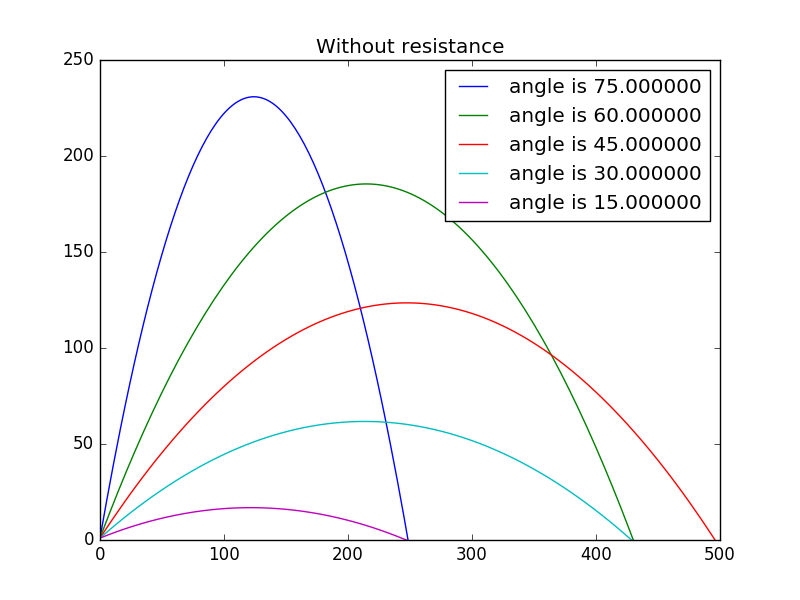$15^\circ$,$30^\circ$,$45^\circ$,$60^\circ$and $75^\circ$.

5.2 Difference with or without resistance

With the intial angle being $45^\circ$, the mass being $10 kg$, velocity component being $50m/s$. The difference in resistance is shown in the track as:

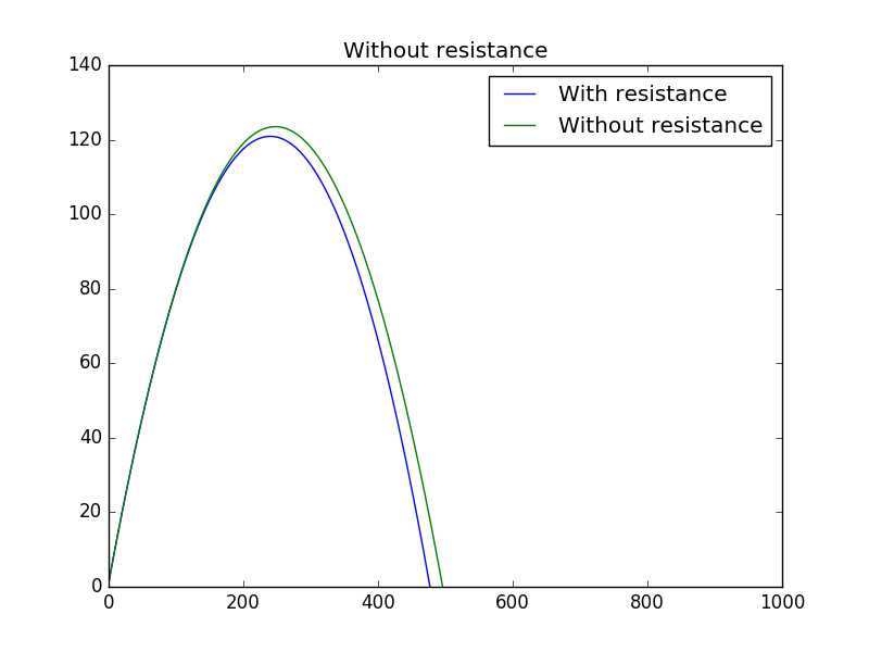
It is obvious that the green one is with resistance,and its maxium height and ranges become smaller as the ideal one.In the above figure,we set $B_{1}=B_{2}=0.001$.

Now we change the parameter$B_{1}=B_{2}=0.01$,you can see the difference even more clearly.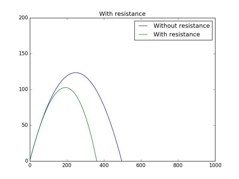

5.3 Difference with resistance and isothermal effect

We set $F_{0}=500N$,and $B_{1}=B_{2}=0.001$

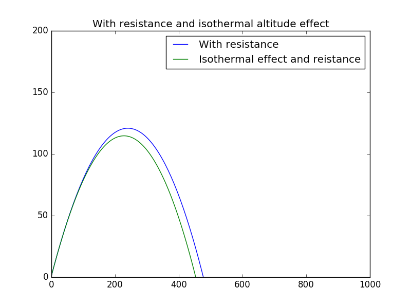
From the above figure,we see in the isothermal situation,the track changes slightly before the maxium height,but differes greatly after the maxium height.

5.4 Difference with isothermal,adibatic and none effect

Here we set $F_{0}=50N$, $B_{1}=B_{2}=0.001$

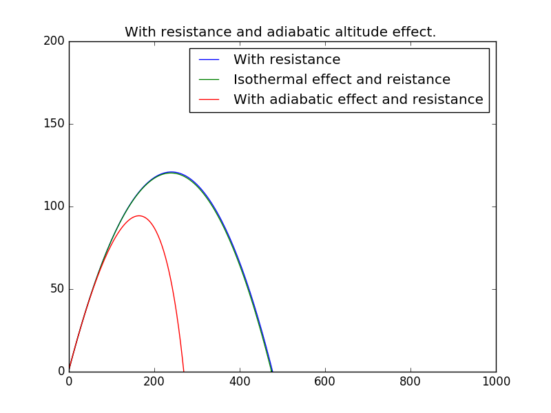
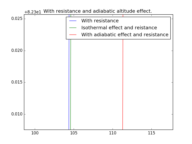
It is evidently that the adiabatic process decrease greatly than the isothermal effect,and shows a characteristic of unsymmertic.

To make the difference even more clearly,I amplify the details to show:

5.5 Difference with or without gravational variation.

$v=50\sqrt{2}m/s$, $F_{0}=50N$, $B_{1}=B_{2}=0.001$

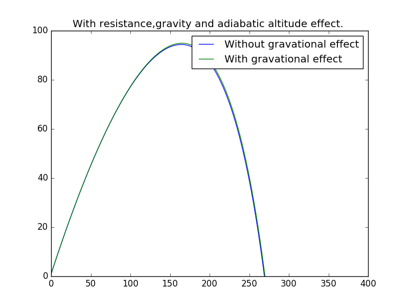
As the altitude isn't so high,the gravation constant $g$ almost remains constan,which means little variation in the figure,just as we have expected!

5.6 Difference of all

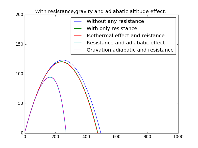
And the detailed one:

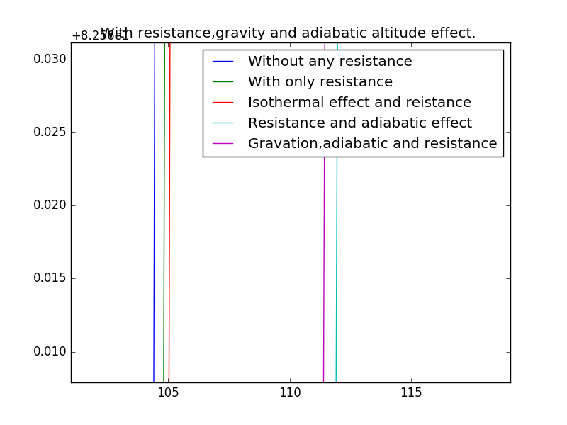
(In the previous without gravational effect,we set $g=10m/s^{2}$,so there may be some faluts with the last two rows.)

6 Acknowlegement

1.Matplotlib
2.Computational Physics
3.Tutorial-Chapter 2 Realistic Projectile Motion