1.Problem

1.5 on Textbook page 16.

2.Abstract

In this passage,we are going to talk about a numerical problem called the decay betweeen A and B.With the preceeding knowledge of matplotlib and the Euler method to calcualte the numerical problem.

3.Background Introduction

As is known to all that the great mathematician Euler had developed a simple but useful way to calculate the numerical problem by using the Taylor expansion.

Euler method:

$$\begin{eqnarray*} \frac{dN_U}{dt}=\frac{N_U(t+\Delta t)-N_U(t)}{\Delta t} \end{eqnarray*}$$
Here,in the discussion of the double decay problem,we again use this method to solve this problme out.Simple and beautiful.We can simulate different situations by inputting different intial conditions,which is very convenient for us to observe subtle differences.Additionally,we are going to discuss the precesion of the plot in details.

4.Main

import pylab as pl
import time
class calcualtion_of_decay(object):
    def __init__(self,time_constant=1,duration=10,number_of_nuclei_A=100,number_of_nuclei_B=0,time_step=0.002):
        self.n_uranium_A=[number_of_nuclei_A]
        self.n_uranium_B=[number_of_nuclei_B]
        self.t=[0]
        self.tau=time_constant
        self.steps=int(duration//time_step+1)
        self.dt=time_step
        self.time=duration
        print('Initial number of nuclei A is',number_of_nuclei_A)  
        print('Initial number of nuclei B is',number_of_nuclei_B)    
        print('Duration is(second)',duration)
        print('Time steps is',time_step)
        print('Time constant is',time_constant)
    def calculate(self):
        for i in range(self.steps):
            tmp_A=self.n_uranium_A[i]+(self.n_uranium_B[i]/self.tau-self.n_uranium_A[i]/self.tau)*self.dt
            tmp_B=self.n_uranium_B[i]+(self.n_uranium_A[i]/self.tau-self.n_uranium_B[i]/self.tau)*self.dt
            self.n_uranium_A.append(tmp_A)
            self.n_uranium_B.append(tmp_B)
            self.t.append(self.t[i]+self.dt)
    def show(self):
        pl.plot(self.t,self.n_uranium_A,'r',label='Nuclei A')
        pl.plot(self.t,self.n_uranium_B,'g',label='Nuclei B')
        pl.xlabel('time s')
        pl.ylabel('Number of nuclei')
        pl.xlim(0.0,4)
        pl.title('The decay of Nuclei A and B,steps is %s'%self.dt')
        pl.show()
        pl.legend()
        def store_results(self):
        myfile = open('nuclei_decay_data.txt', 'w')
        for i in range(len(self.t)):
            print(self.t[i], self.n_uranium[i], file = myfile)
        myfile.close()
print('This program is going to show you the decay of Nuclei A and B')
x1=input('Please input the time constant' '\n')
x2=input('Please input the time duration' '\n')
x3=input('Please input the intial number of Nuclei A' '\n')
x4=input('Please input the intial number of Nuclei B' '\n')
x5=input('Please input the steps(the smaller you input,the more precise plot you get!)' '\n')
a=calcualtion_of_decay(x1,x2,x3,x4,x5)
a.calculate()
a.show()

5.Result

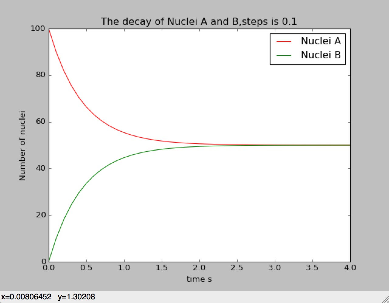
Situation 1:

Parameter:
Number fo Nuclei A is 100
Number of Nuclei B is 0
Time constant is 1s
Steps is 0.1

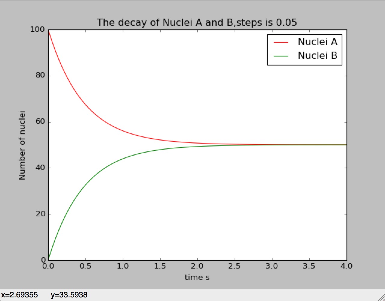
Situation 2:

Parameter:
Number fo Nuclei A is 100
Number of Nuclei B is 0
Time constant is 1s
Steps is 0.05

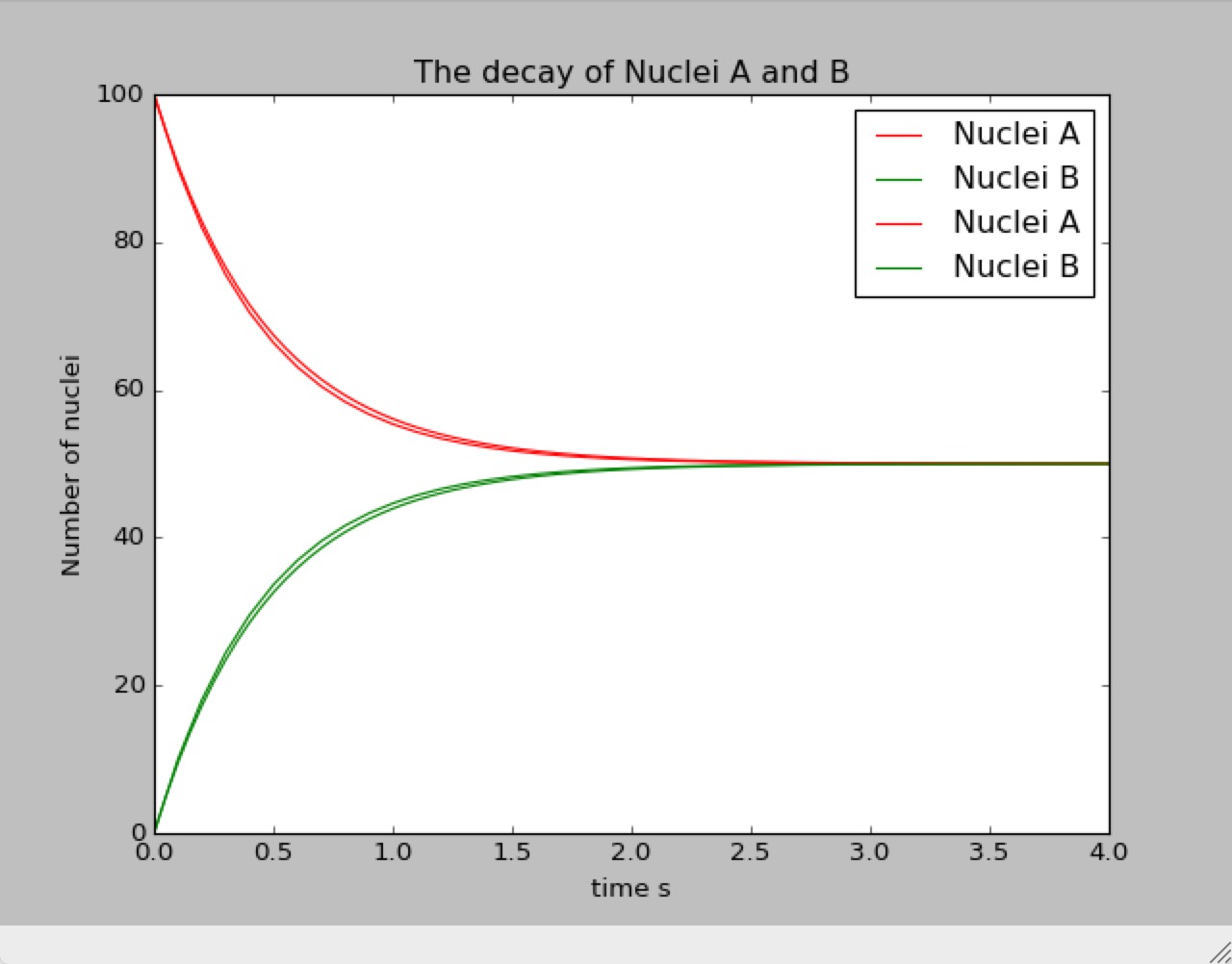
Situation 3：

Comparison between steps=0.1 and steps=0.5

Situation 4:

Comparison between steps=0.1 and steps=0.001

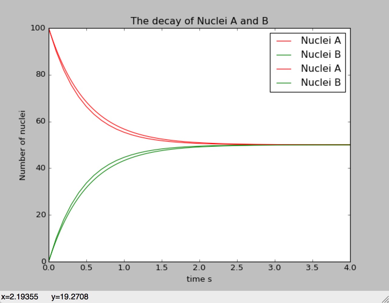
The more detailed picture:

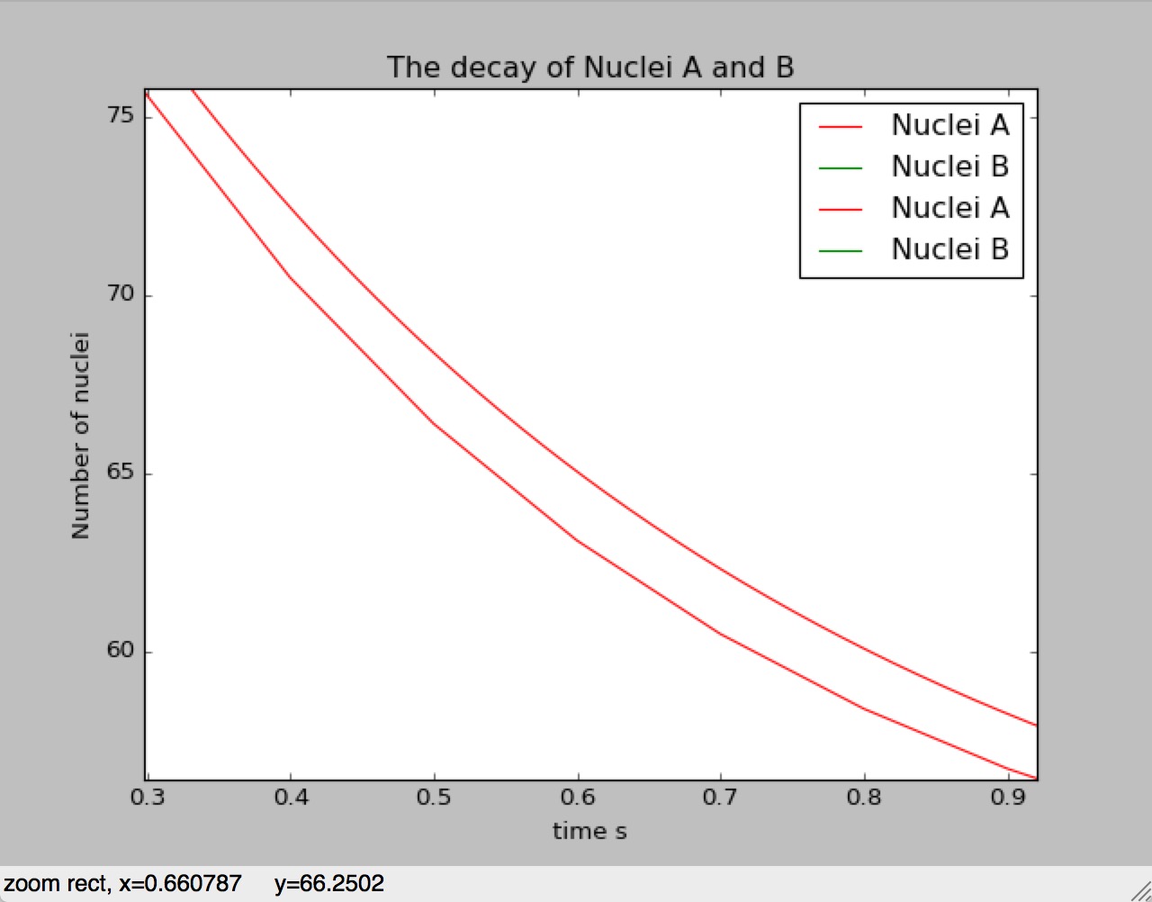
6.Discussion

In part 5 we see,that the smaller the steps is,the lower the plot is going to be than the bigger one.Owing to the o($t^{2}$) term is omitted,and the square-term is always positive,so,as the steps is becoming smaller,the positive term is become lesser.That's the reason why there will be a derivation in the picture with different precesion.

7.Acknowldegment

1.Tutorial_Chapter 1 A First Numerical Problem
2.Matplotlib.com