生成对抗网络：CGAN，InfoGAN

MachineLearning

---

1、CGAN

这个真的是好简单呃…但是效果出奇的好。

https://blog.csdn.net/liuxiao214/article/details/73485333
https://zhuanlan.zhihu.com/p/44170959
https://zhuanlan.zhihu.com/p/25542274

1.1 基本思想

传统GAN，特别是生成器，在生成的时候，往往会生成很多随机的内容（毕竟输入就是个随机向量，还想怎么样）。现在人们想通过给生成器一定的约束，让它能够在生成的时候有一点规律。

放到公式里，就是这样：
传统GAN

$$\underset{G}{min}~\underset{D}{max} V(G,D)=E_{x-p_{data}}[log(D(x))]+E_{x-p_{G(z)}}[log(1-D(x))]$$
CGAN
$$\underset{G}{min}~\underset{D}{max} V(G,D)=E_{x-p_{data}}[log(D(x|y))]+E_{x-p_{G(z)}}[log(1-D(x|y))]$$

即，我们需要求在给定条件y的情况下，D和G的最优解。

那么y是什么呢：

1、对于生成器而言，就是这次你希望生成器生成的内容满足一个什么样的条件。
   在之前有的例子是生成二次元萌妹的，没有任何约束的时候，生成的都是随机的妹子；但是CGAN中，如果你让y=‘金发碧眼’，那么生成的所有妹子都是金发碧眼。
2、对于判别器而言，在没有y之前，只需要判断这个是生成数据还是真实数据。但是现在，生成器起到了一点分类器的作用：
    2.1 对于真实数据，他不仅要判断这是一个真实数据，还需要判断这个真实数据是不是满足输入条件y。
    2.2 对于生成数据，他要在输入约束y的条件下，去判断这个x是不是生成数据。

1.2 网络结构

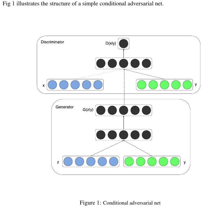
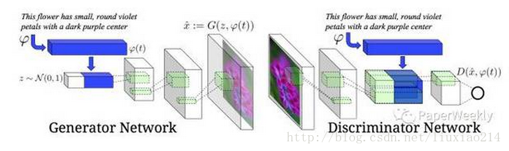
这个图也许不够清楚，那么看看下面这个：

网上的文章说的很少，我一开始还以为是没人看，结果是太简单了。

什么条件概率啥的，放到网络里，就是无脑拼接= -。

1.3 改进策略

感觉CGAN和InfoGAN就是除了随机噪声外，还加入一些隐变量，然后通过一些办法，让隐变量起作用。

当然，为了让模型更好的训练，作者还加入了一些调优策略。

• 1）针对判别器改进。之前说了判别器需要判断图像是真实还是生成，以及是否满足描述，而原来我们的数据只有两种： a. 真实数据+正确label；b. 生成数据+正确label。现在，作者还加入了：c. 真实数据+错误label。通过这样的方式，来加速判别器的训练和收敛。

• 2）其实我感觉针对判别器的这一套改进才是重点。若是对输入的label内容没有任何的使用，它的效果不会很好（或者直接丢给你一个和原始GAN一样的网络也不是不行）。但是由于在判别器中，我们加入了对LABEL的判断，尤其是对【真实数据+错误label】数据的加入，令整个网络能够学习并使用这个附加内容。

• 3）针对生成器改进。这里就是用扩展数据集的方式，设一个文字描述是$\varphi(t_1)$，另一个文字描述是$\varphi(t_2)$，我们可以得到他们的一个内插值$\beta\varphi(t_1) + (1-\beta)\varphi(t_1)$。其中$0<\beta<1$。这样的内插实际上是得到了两个文字描述的某种“中间态”，为我们增加了样本数量。

1.4 搭建网络

算来算去，这是我写的第一个GAN，先上效果图：(左边是初始状态，右边CPU跑了1000轮）

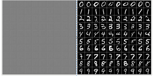
下面代码静下心来看看，应该很好看懂，不想静心的话，可以直接看看训练部分，弄清楚每个输入数据的格式，shape，就能够大概明白整个流程。

代码：

# load data
from tensorflow.examples.tutorials.mnist import input_data
# 把mnist数据放在MNIST_data下就好
mnist = input_data.read_data_sets('MNIST_data',one_hot=True)
OUTPUT_DIR='samples'
if not os.path.exists(OUTPUT_DIR):
    os.mkdir(OUTPUT_DIR)
tf.reset_default_graph()
X = tf.placeholder(dtype=tf.float32, shape=[None, HEIGHT, WIDTH, 1], name='X')
y_label = tf.placeholder(dtype=tf.float32, shape=[None, HEIGHT, WIDTH, LABEL], name='y_label')
noise = tf.placeholder(dtype=tf.float32, shape=[None, z_dim], name='noise')
y_noise = tf.placeholder(dtype=tf.float32, shape=[None, LABEL], name='y_noise')
is_training = tf.placeholder(dtype=tf.bool, name='is_training')
def lrelu(x,leak=0.2):
    return tf.maximum(x,leak*x)
def sigmoid_cross_entropy_with_logits(x,y):
    return tf.nn.sigmoid_cross_entropy_with_logits(logits=x,labels=y)
# discriminator
def discriminator(image,label,reuse=None,is_training=is_training):
    momentum=0.9
    with tf.variable_scope('discriminator',reuse=reuse):
        # 把输入图像和condition进行拼接 【无脑拼接】
        h0 = tf.concat([image,label],axis=3)
        h0 = tf.layers.conv2d(h0,kernel_size=5,filters=64,strides=2,padding='same')
        h0 = lrelu(h0)
        # 对于batch_norm，训练的时候需要，推断的时候就不需要。
        h1 = tf.layers.conv2d(h0,kernel_size=5,filters=128,strides=2,padding='same')
        h1 = lrelu(tf.contrib.layers.batch_norm(h1,is_training=is_training,decay=momentum))
        h2 = tf.layers.conv2d(h1,kernel_size=5,filters=256,strides=2,padding='same')
        h2 = lrelu(tf.contrib.layers.batch_norm(h2,is_training=is_training,decay=momentum))
        h3 = tf.layers.conv2d(h2,kernel_size=5,filters=512,strides=2,padding='same')
        h3 = lrelu(tf.contrib.layers.batch_norm(h3,is_training=is_training,decay=momentum))
        # 最后一层输出拉平+全连接，没有用FCN。
        h4 = tf.contrib.layers.flatten(h3)
        h4 = tf.layers.dense(h4,units=1)
        # h4是一个batch_size*1的向量吧
        return tf.nn.sigmoid(h4),h4
# generator
def generator(z,label,is_training=is_training):
    momentum=0.9
    with tf.variable_scope('generator',reuse=None):
        d =3
        z = tf.concat([z,label],axis=1)
        h0 = tf.layers.dense(z,units=d*d*512)
        h0 = tf.reshape(h0,shape=[-1,d,d,512])
        h0 = tf.nn.relu(tf.contrib.layers.batch_norm(h0,is_training=is_training,decay=momentum))
        h1 = tf.layers.conv2d_transpose(h0,kernel_size=5,filters=256,strides=2,padding='same')
        h1 = tf.nn.relu(tf.contrib.layers.batch_norm(h1,is_training=is_training,decay=momentum))
        h2 = tf.layers.conv2d_transpose(h1,kernel_size=5,filters=128,strides=2,padding='same')
        h2 = tf.nn.relu(tf.contrib.layers.batch_norm(h2,is_training=is_training,decay=momentum))
        h3 = tf.layers.conv2d_transpose(h2,kernel_size=5,filters=64,strides=2,padding='same')
        h3 = tf.nn.relu(tf.contrib.layers.batch_norm(h3,is_training=is_training,decay=momentum))
        h4 = tf.layers.conv2d_transpose(h3,kernel_size=5,filters=1,strides=1,
                                        padding='valid',activation=tf.nn.tanh,name='g')
        return h4
# loss
# 1、拿到生成的生成内容
g = generator(noise, y_noise)
# 2、用真实数据训练判别器
d_real, d_real_logits = discriminator(X, y_label)
# 3、用生成数据训练判别器
d_fake, d_fake_logits = discriminator(g, y_label, reuse=True)
# 喵喵喵？？？
vars_g = [var for var in tf.trainable_variables() if var.name.startswith('generator')]
vars_d = [var for var in tf.trainable_variables() if var.name.startswith('discriminator')]
# 4、通过判别器拿到V（G，D）中第一项
loss_d_real=tf.reduce_mean(sigmoid_cross_entropy_with_logits(d_real_logits,tf.ones_like(d_real)))
# 5、通过判别器拿到V（G，D）中第二项
loss_d_fake=tf.reduce_mean(sigmoid_cross_entropy_with_logits(d_fake_logits,tf.zeros_like(d_fake)))
# 6、通过判别器定义生成器的loss
loss_g=tf.reduce_mean(sigmoid_cross_entropy_with_logits(d_fake_logits,tf.ones_like(d_fake)))
# 7、组合得到判别器的loss
loss_d=loss_d_fake+loss_d_real
# optimizer
update_ops = tf.get_collection(tf.GraphKeys.UPDATE_OPS)
with tf.control_dependencies(update_ops):
    optimizer_d = tf.train.AdamOptimizer(learning_rate=0.0002,beta1=0.5).minimize(loss_d,var_list=vars_d)
    optimizer_g = tf.train.AdamOptimizer(learning_rate=0.0002,beta1=0.5).minimize(loss_g,var_list=vars_g)
# 就是为了方便看结果，和模型没关系
def montage(images):
    if isinstance(images,list):
        images = np.array(images)
    img_h = images.shape[1]
    img_w = images.shape[2]
    n_plots = int(np.ceil(np.sqrt(images.shape[0])))
    m = np.ones((images.shape[1]*n_plots+n_plots+1,images.shape[2]*n_plots+n_plots+1))*0.5
    for i in range(n_plots):
        for j in range(n_plots):
            this_filter = i*n_plots+j
            if this_filter < images.shape[0]:
                this_img = images[this_filter]
                m[1 + i + i * img_h:1 + i + (i + 1) * img_h,
                  1 + j + j * img_w:1 + j + (j + 1) * img_w] = this_img
    return m
sess=tf.Session()
sess.run(tf.global_variables_initializer())
z_samples = np.random.uniform(-1.0,1.0,[batch_size,z_dim]).astype(np.float32)
y_samples = np.zeros([batch_size,LABEL])
for i in range(LABEL):
    for j in range(LABEL):
        y_samples[i*LABEL+j,i]=1
samples=[]
loss={'d':[],'g':[]}
import time
'''
batch_size=100
z_dim=100
WIDTH=28
HEIGHT=28
LABEL=10
'''
for i in tqdm(range(60000)):
    # 0、generator每次也就100个输入，每个输入为长100的向量
    n = np.random.uniform(-1.0,1.0,[batch_size,z_dim]).astype(np.float32)
    # 1、拿到的训练集图片，像素值已经被归一化到0~1之间
    batch,label=mnist.train.next_batch(batch_size=batch_size)
    #  1.1 从batch_size,784 reshape到 batch_size,28,28; 最后那个1表示channel
    batch = np.reshape(batch,[batch_size,HEIGHT,WIDTH,1])
    #  1.2 将0~1的图像像素值变成-1~1之间，满足tanh的要求。
    batch = (batch-0.5)*2
    yn = np.copy(label)
    # 2、能够理解这么做是为了在判别器中将label和图片接在一起，只是这种做法有点迷= -
    # label从 batch，1,1，LABEL_LEN的张量，变成，batch,28,28,LABEL_LEN的张量
    y1 = np.reshape(label,[batch_size,1,1,LABEL])
    y1 = y1*np.ones([batch_size,HEIGHT,WIDTH,LABEL])
    # 3、先跑一下loss，保存loss结果，为了后面画图用
    d_ls,g_ls = sess.run([loss_d,loss_g],feed_dict={X:batch,noise:n,y_label:y1,
                                                    y_noise:yn,is_training:True})
    loss['d'].append(d_ls)
    loss['g'].append(g_ls)
    # 4、真正训练在这里，基本就是判别器训练一次，生成器训练2次。
    #  4.1 其实可以这么理解，训练一次判别器，需要真实数据（batch），以及生成器生成的数据。
    #  4.2 而生成器一次就只生成batch_size大小的数据。
    #  4.3 因此判别器一次训练，所使用的数据量，是判别器的两倍，所以训练一次判别器，需要训练两次生成器。
    sess.run(optimizer_d,feed_dict={X: batch, noise: n, y_label: y1, 
                                    y_noise: yn, is_training: True})
    sess.run(optimizer_g, feed_dict={X: batch, noise: n, y_label: y1,
                                     y_noise: yn, is_training: True})
    sess.run(optimizer_g, feed_dict={X: batch, noise: n, y_label: y1, 
                                     y_noise: yn, is_training: True})
    if i % 1000 == 0:
        print(i, d_ls, g_ls)
        # 5、每次到了节点，把这个时刻生成器生成的内容输出一下。
        gen_imgs = sess.run(g, feed_dict={noise: z_samples, y_noise: y_samples, 
                                          is_training: False})
        # 6、生成器输出的图像，像素在-1~1之间，现在需要把它们转化回0~1之间。
        gen_imgs = (gen_imgs + 1) / 2
        # 7、逐个拿一下图片，拼图啥的。
        imgs = [img[:, :, 0] for img in gen_imgs]
        gen_imgs = montage(imgs)
        plt.axis('off')
        plt.imshow(gen_imgs, cmap='gray')
        imageio.imsave(os.path.join(OUTPUT_DIR, 'sample_%d.jpg' % i), gen_imgs)
        plt.show()
        samples.append(gen_imgs)
plt.plot(loss['d'], label='Discriminator')
plt.plot(loss['g'], label='Generator')
plt.legend(loc='upper right')
plt.savefig('Loss.png')
plt.show()
imageio.mimsave(os.path.join(OUTPUT_DIR, 'samples.gif'), samples, fps=5)
saver = tf.train.Saver()
saver.save(sess, './mnist_cgan', global_step=60000)

使用生成器

import tensorflow as tf
import numpy as np
import matplotlib.pyplot as plt
batch_size = 100
z_dim = 100
LABEL = 10
def montage(images):
    if isinstance(images, list):
        images = np.array(images)
    img_h = images.shape[1]
    img_w = images.shape[2]
    n_plots = int(np.ceil(np.sqrt(images.shape[0])))
    m = np.ones((images.shape[1] * n_plots + n_plots + 1, images.shape[2] * n_plots + n_plots + 1)) * 0.5
    for i in range(n_plots):
        for j in range(n_plots):
            this_filter = i * n_plots + j
            if this_filter < images.shape[0]:
                this_img = images[this_filter]
                m[1 + i + i * img_h:1 + i + (i + 1) * img_h,
                  1 + j + j * img_w:1 + j + (j + 1) * img_w] = this_img
    return m
sess = tf.Session()
sess.run(tf.global_variables_initializer())
saver = tf.train.import_meta_graph('./mnist_cgan-60000.meta')
saver.restore(sess, tf.train.latest_checkpoint('./'))
graph = tf.get_default_graph()
g = graph.get_tensor_by_name('generator/g/Tanh:0')
noise = graph.get_tensor_by_name('noise:0')
y_noise = graph.get_tensor_by_name('y_noise:0')
is_training = graph.get_tensor_by_name('is_training:0')
n = np.random.uniform(-1.0, 1.0, [batch_size, z_dim]).astype(np.float32)
y_samples = np.zeros([batch_size, LABEL])
for i in range(LABEL):
    for j in range(LABEL):
        y_samples[i * LABEL + j, i] = 1
gen_imgs = sess.run(g, feed_dict={noise: n, y_noise: y_samples, is_training: False})
gen_imgs = (gen_imgs + 1) / 2
imgs = [img[:, :, 0] for img in gen_imgs]
gen_imgs = montage(imgs)
plt.axis('off')
plt.imshow(gen_imgs, cmap='gray')
plt.show()

2、InfoGAN

https://blog.csdn.net/dagekai/article/details/53953513
https://blog.csdn.net/u011699990/article/details/71599067
https://www.jianshu.com/p/b8c34c6f09ad

2.1 基本理论

对于原始的GAN而言，生成器的输入z和输出x之间，是没有什么可解释性的。即，我们不知道什么样的z能够生成什么样的x。

在CGAN中，我们通过给定一个隐向量c，以及让判别器去判断生成/真实图像是否符合描述，来约束生成器的行为。这一定程度上，可以认为是，描述c控制了输出x中的与c相关的特征。

然后，呃，有的大佬或许觉得这样不过瘾吧，说我想控制所有的特征；然而我并不能知道一幅图像有哪些特征。于是，我给一个向量作为隐向量，和GAN网络一起训练，然后可以认为，这个向量的每一维，都描述了图像的某一种特征。

问题：

对于这样的隐向量，我没有办法知道它到底描述的是哪几个特征，因此没办法使用CGAN里面的策略来判断这个隐向量是否生效了。

解决：

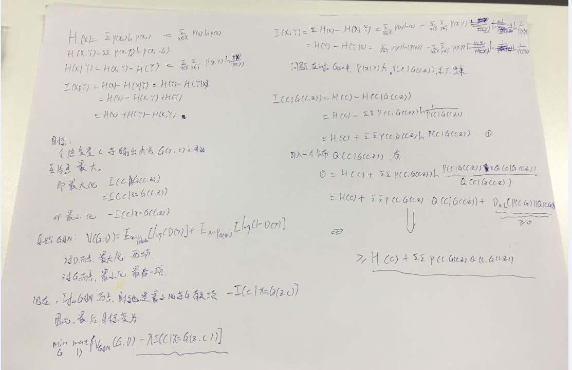
隐向量最直接的影响应该是生成器的输出，那么只要判断隐向量和生成器输出之间的互信息，就能够知道隐向量是否起作用了。

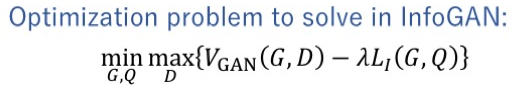
最终的COST——function：其中L1是经过优化的互信息下界。

详细推断：

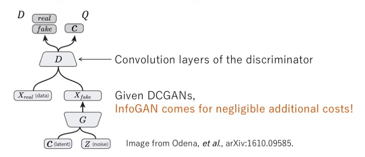
2.2 网络结构

网络的逻辑结构就是这样，具体的结构可以和CGAN差不多。

2.3 具体实现

网上找的一版感觉有点问题= -，之后试试keras版本的。