第十一讲 波动率模型及应用（II）

樊潇彦 复旦大学经济学院 金融数据

---

下载：Ch11_Data.rar

# 准备工作
setwd("D:\\...\\Ch11")
## 调用
library(fGarch)
library(rugarch)
library(tidyverse)
library(readxl)
library(ggplot2)
library(tseries)
library(zoo)
library(forecast)

3. GARCH模型（续）

3.4 指数GARCH模型（EGARCH）

考虑到正的和负的资产收益率的非对称效应，Nelson(1991)提出了指数GARCH(m,n)模型：

$${r_t} = \mu + {\varepsilon _t}\\ {\varepsilon _t} = {\sigma _t}{z_t}\\ ln(\sigma _t^2) = \omega + \sum\limits_{s = 1}^m {\left[ {{\alpha _s}{z_{t - s}} + \gamma_s \left( {\left| {{z_{t - s}}} \right| - E\left| {{z_{t - s}}} \right|} \right)} \right]} + \sum\limits_{s = 1}^n {{\beta _s}ln(\sigma _{t - s}^2)}$$

注：Tsay(2015，P171)第二行：

$$ln(\sigma _t^2) = \omega + \gamma_1 \left({\alpha _1} {{z_{t - 1}} + {\left| {{z_{t - 1}}} \right|} } \right) + {\beta _1}ln(\sigma _{t - 1}^2)$$

与GARCH模型相比，EGARCH模型有两点改进：
1. 使用对数条件方差，放松了对模型系数非负性的限制；
2. 股价上升/下跌（$z_t$ 为正/负）对模型的影响不对称。当 $\alpha_s<0$ 时，价格下跌（$z_{t-s}<0$）将使资产波动率上升，存在杠杆效应。

• 例1：苹果公司股票

load("AAPL.RData")
colnames(AAPL)
ret.aapl=diff(log(zooreg(AAPL)$AAPL.Close))              # 计算收益率
plot(ret.aapl)
egarch11.spec = ugarchspec(
  variance.model = list(model="eGARCH", garchOrder=c(1,1)), 
  mean.model = list(armaOrder=c(0,0)))                   # 设定EGARCH(1,1)模型
aapl.egarch11.fit = ugarchfit(spec=egarch11.spec, data=ret.aapl)
aapl.egarch11.fit
plot(aapl.egarch11.fit,which=12)                         # 冲击影响非对称，存在杠杆效应
# 与GARCH(1,1)模型比较
garch11.spec = ugarchspec(
  variance.model =list(model="sGARCH", garchOrder=c(1,1)), 
  mean.model = list(armaOrder=c(0,0)))                   
aapl.garch11.fit = ugarchfit(spec=garch11.spec, data=ret.aapl)
plot(aapl.garch11.fit,which=12)                          # 冲击影响对称，没有杠杆效应

• 例2：IBM股票

# P171（4-34）式
source("Egarch.R") 
da=read.table("m-ibmsp6709.txt",header=T) 
head(da)  
ibm=log(da$ibm+1) 
Box.test(ibm,lag=12,type='Ljung')
m1=Egarch(ibm) 
# 用rugarch包中命令回归
egarch11.spec= ugarchspec(
  variance.model =list(model="eGARCH", garchOrder=c(1,1)), 
  mean.model = list(armaOrder=c(0,0),include.mean=T))                   
ibm.egarch11.fit = ugarchfit(spec=egarch11.spec, data=ibm)
ibm.egarch11.fit

3.5 门限GARCH模型（TGARCH）

• Glosten et al.(1993)，又称为GJR-GARCH模型。当 $\gamma_s>0$ 时，存在杠杆效应:
  $${\sigma _t^2 = \omega + \sum\limits_{s = 1}^m {({\alpha _s} + {\gamma _s}{N_{t - s}})\varepsilon _{t - s}^2} + \sum\limits_{s = 1}^n {{\beta _s}\sigma _{t - s}^2} }\\{N_{t - s}} = \left\{ {\begin{array}{*{20}{c}} {1,~{\varepsilon _{t - s}} < 0}\\ {0,~{\varepsilon _{t - s}} \ge 0} \end{array}} \right.$$
• Zakoian(1994):
  $${{\sigma _t} = \omega + \sum\limits_{s = 1}^m {{\alpha _s}(\left| {{\varepsilon_{t - s}}} \right| + {\gamma _s}{\varepsilon_{t - s}})} + \sum\limits_{s = 1}^n {{\beta _s}{\sigma _{t - s}}} }$$

# 欧元兑美元汇率数据，P174：（4-36）式
da=read.table("d-useu9910.txt",header=T)
eu=diff(log(da$rate))*100
source('Tgarch11.R')  # 原文件中 filter 命令前加上 stats::
m1=Tgarch11(eu)
# 用rugarch包中命令回归
tgarch11.spec = ugarchspec(
  variance.model = list(model="gjrGARCH", garchOrder=c(1,1)), # GJR模型
  mean.model = list(armaOrder=c(0,0),include.mean=T))
eu.tgarch11.fit = ugarchfit(spec=tgarch11.spec, data=eu)
eu.tgarch11.fit
# TGARCH杠杆效应作图
plot(eu.tgarch11.fit, which=12)

3.6 非对称幂ARCH模型（APARCH）

$$\sigma^\delta_t = \omega + \sum\limits_{s = 1}^m{\alpha_s(|\varepsilon_{t-s}|-\gamma_s\varepsilon_{t-s})^\delta}+\sum\limits_{s = 1}^n{\beta_s\sigma^\delta_{t-s}}$$

• $\delta=2$：Glosten et al.(1993)TGARCH模型，也称GJR-GARCH模型
• $\delta=1$：Zakoia(1994)TGARCH模型
• $\delta=0$：EGARCH模型

# P175：汇率数据的APARCH模型
m1=garchFit(~1+aparch(1,1),data=eu,trace=F)
summary(m1)
m2=garchFit(~1+aparch(1,1),data=eu,trace=F,delta=2,include.delta=F) # delta=2, TGARCH(1,1)模型
summary(m2)
# 用rugarch包中命令回归
aparch11.spec = ugarchspec(
  variance.model = list(model="apARCH", garchOrder=c(1,1)),    
  mean.model = list(armaOrder=c(0,0),include.mean=T))
eu.aparch11.fit = ugarchfit(spec=aparch11.spec, data=eu)
# APARCH杠杆效应作图
plot(eu.aparch11.fit, which=12)

3.7 非对称GARCH模型（NGARCH 或 AGARCH）

$$\sigma^2_t = \omega + \sum\limits_{s = 1}^m{\alpha_s\sigma^2_{t-s}(z_{t-s}-\eta_{s})^2}+\sum\limits_{s = 1}^n{\beta_s\sigma^2_{t-s}}$$

# P178：（4-41）式
source("Ngarch.R")
m1=Ngarch(eu)
summary(m1)
# 用rugarch包中命令回归
ngarch11.spec = ugarchspec(
  variance.model = list(model="fGARCH",submodel = "NAGARCH", garchOrder=c(1,1)),    
  mean.model = list(armaOrder=c(0,0)))
eu.ngarch11.fit = ugarchfit(spec=ngarch11.spec, data=eu)
# NGARCH杠杆效应作图
plot(eu.ngarch11.fit, which=12) 

4. 用高频率数据估计波动率

高频数据包括两种：一是每天同一价格（如收盘价），另一种是每天开盘、最高、最低、收盘（OHLC）四种价格，这两种高频的日度数据都可以用来计算低频的月度（或年度）收益率。用 TTR 包中的 volatility(OHLC, calc = "close", n = 10, N = 260, ...) 命令可以轻松实现，其中 n 为天数，N 为一年的交易日数，calc 为不同的估计方法，具体包括：

• close，Close-to-Close Volatility.
  $$\sigma = \sqrt{\frac{N}{n-2} \sum_{i=1}^{n-1}(r_i-\bar{r})^2} \\ r_i=\ln\left(\frac{C_{i+1}}{C_i}\right),~~\bar{r} = \frac{r_1+r_2+\ldots r_{n-1}}{n-1}$$
• parkinson，Parkinson(1980) High-Low Volatility.
  $$\sigma = \sqrt{\frac{N}{4n \ln2}\sum_{i=1}^{n}\left(\ln \frac{H_i}{L_i}\right)^2}$$
• garman.klass，Garman and Klass(1980) assumes Brownian motion with zero drift and no opening jumps (i.e. the opening = close of the previous period).
  $$\sigma = \sqrt{ \textstyle\frac{N}{n} \sum \left[ \left( \ln \textstyle\frac{O_i}{C_{i-1}} \right)^2 + \textstyle\frac{1}{2}\displaystyle \left( \ln \textstyle\frac{H_i}{L_i} \right)^2 - (2\ln 2-1) \left( \ln\textstyle\frac{C_i}{O_i} \right)^2 \right]}$$
• rogers.satchell，Rogers and Satchell(1991) allows for non-zero drift, but assumed no opening jump.
  $$\sigma = \sqrt{ \textstyle\frac{Z}{n} \sum \left[ \ln \textstyle\frac{H_i}{C_i} \ln \textstyle\frac{H_i}{O_i} + \ln \textstyle\frac{L_i}{C_i} \ln \textstyle\frac{L_i}{O_i} \right]}$$
• yang.zhang，Yang and Zhang(2000) has minimum estimation error, and is independent of drift and opening gaps. It can be interpreted as a weighted average of the Rogers and Satchell estimator, the close-open volatility, and the open-close volatility.
  $$\begin{align*} \sigma^2 &= \sigma_o^2 + k\sigma_c^2 + (1-k)\sigma_{rs}^2\\ \\ \sigma_o^2 &=\textstyle \frac{N}{n-1} \sum\left( \ln\frac{O_i}{C_{i-1}}-\mu_o \right)^2,~~\mu_o=\textstyle \frac{1}{n} \sum \ln\frac{O_i}{C_{i-1}}\\ \sigma_c^2 &=\textstyle \frac{N}{n-1} \sum\left( \ln\frac{C_i}{O_i}-\mu_c \right)^2,~~\mu_c=\textstyle \frac{1}{n} \sum \ln\frac{C_i}{O_i}\\ \sigma_{rs}^2 &= \textstyle\frac{N}{n} \sum \left( \ln \textstyle\frac{H_i}{C_i} \ln \textstyle\frac{H_i}{O_i} + \ln \textstyle\frac{L_i}{C_i} \ln \textstyle\frac{L_i}{O_i} \right) \\ k&=\frac{0.34}{1+\frac{n+1}{n-1}} \end{align*}$$

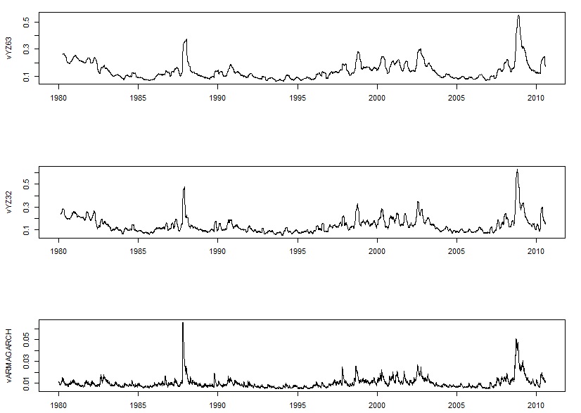
da=read.table("d-sp58010.txt",header=T)                     # 1980-2010年S&P500数据
head(da)
ohlc <- da[,c("Open","High","Low","Close")]
library(TTR)
vClose <- volatility(ohlc, calc="close")
plot(vClose,type="l")
par(mfcol=c(3,1))
tdx=c(1:7737)/253+1980
vYZ63 <- volatility(ohlc, calc="yang.zhang", n=63, N=252)   # 窗口为63期
plot(x=tdx,vYZ63,type="l",xlab="")
vYZ32 <- volatility(ohlc, calc="yang.zhang", n=32, N=252)   # 窗口为32期
plot(x=tdx,vYZ32,type="l",xlab="")
cl=da[,"Close"]
rtn=diff(log(cl))                                           # 计算收盘价对数回报率
armagarch= ugarchspec(
  variance.model = list(model="sGARCH", garchOrder=c(1,1)), 
  mean.model = list(armaOrder=c(4,0),include.mean=T))
fitted=ugarchfit(spec=armagarch, data=rtn)                  # P186：ARMA-GARCH模型
names(fitted@fit)                                           # 查看估计结果的名称
vARMAGARCH=fitted@fit$sigma
plot(x=tdx[-1],vARMAGARCH,type="l",xlab="")                 # sigma作图

5. 波动率预测

aapl.garch11.fit = ugarchfit(spec=garch11.spec, data=ret.aapl, out.sample=20)
aapl.garch11.fcst = ugarchforecast(aapl.garch11.fit, n.ahead=10, n.roll=10)
plot(aapl.garch11.fcst)
plot(aapl.garch11.fcst, which='all')

课后练习

纽约大学斯特恩商学院波动研究所的波动实验室提供了大量金融数据的建模结果：

• 选一个你感兴趣的金融指标，进行波动率建模分析，并和波动实验室的结果进行比对。
• 观看Prof. Robert Engle 在2020年4月10日的讲座视频 Covid-19 and NYC Series