图的常见算法

java

一、图的基本知识

• 图是节点集合的一个拓扑结构，节点之间通过边相连。图分为有向图和无向图。有向图的边具有指向性，即A - B仅表示由A到B的路径，但不意味着B可以连到A。与之对应的，无向图的每一条边都表示一条双向路径。
  
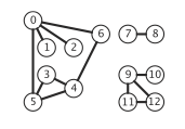
• 连通、连通图：在无向图中，若从顶点v到顶点w 有路径存在则称v和w是连通的。若图G中任意两个顶点都是连通的则称图G是连通图，否则为非连通图。

显然如果一个图有n个顶点，但是边小于n - 1个，则此图肯定是非连通图。

• 极大连通子图，极小连通子图， 连通分量：对于连通图来说，极大连通子图就是其本身，是唯一的。极小就是它的生成树。对于非连通图来说，可以拆成数个极大连通子图，这也就称为联通分量。

• 顶点的度、入度和出度：

  • 每个顶点的度定义为以该顶点为一个端点的边的数目
  • 在具有n个顶点e条边的无向图中，无向图的全部顶点的度之和等于边数的两倍， 即TD(v) = 2e。因为每条边和两个顶点关联
  • 对于有向图，顶点v的度分为入度和出度。入度是以顶点v为终点的有向边的数目，记为ID(v)。出度则是以顶点v 为起点的有向边数目，记为OD(v)。
  • 对于有n个顶点e条边的有向图中，有向图的全部顶点的入度之和与出度之和相等切等于边数，即∑ID(v) = ∑OD(v) = e

二、图的表示

图的表示方式基本有两种，邻接矩阵（adjacency matrix）与邻接表（adjacency list）

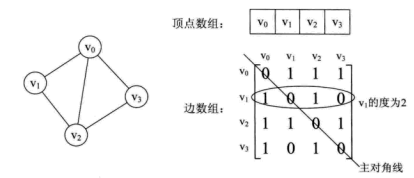
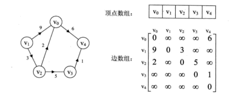
邻接矩阵(adjacency matrix)

下图是无向图和有向图邻接矩阵的表示示意图。

下面给出一个adjecncy matrix 的简单代码表示

public class AdjencyMatrixGraph {
    private int vertic; //the nums of vertices
    private int edge;   //the nums of edges
    private boolean[][] adjencyMatrix;
    public AdjencyMatrixGraph(int vertic) {
        if(vertic < 0)
            throw new RuntimeException("vertices can not be negative");
        this.vertic = vertic;
        edge = 0;
        adjencyMatrix = new boolean[vertic][vertic];
    }
    //add undirected edge v-w
    public void addEdge(int v, int w) {
        if(!adjencyMatrix[v][w]) {
            edge++;
            adjencyMatrix[v][w] = adjencyMatrix[w][v] = true;
        }
    }
    public boolean contain(int v, int w) {
        return adjencyMatrix[v][w];
    }
}

• 无向图的邻接矩阵是对称的，对大规模的adjency matrix可以用压缩矩阵
• 使用adjency matrix很容易确定图中任意两个顶点之间是否有边相连。但是要确定有多少条边则必须按行，列进行搜索遍历，时间复杂度大。因此稠密的图适合用adjency matrix

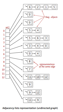
邻接表(adjacency matrix)

下图是无向图和有向图邻接表的表示示意图。

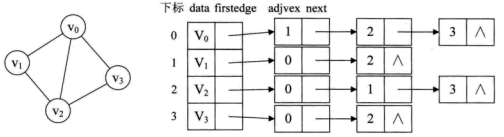
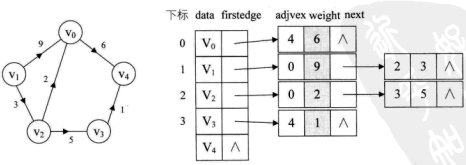
我们设计一个数据结构如下：

下面给出简单代码：

//A single linkedList
public class Bag<T> implements Iterable<T> {
    private class Node<T> {
        T element;
        Node<T> next;
        public Node(T element, Node<T> next) {
            this.element = element;
            this.next = next;
        }
    }
    private Node<T> first;
    private int num;
    public Bag() {
        first = null;
        num = 0;
    }
    public boolean contain(T element) {
        Node<T> cur = first;
        while(cur != null){
            if(element.equals(cur.element)) {
                return true;
            }
            cur = cur.next;
        }
        return false;
    }
    //first insert
    public void add(T element) {
        if(contain(element))    {
            return ;
        }
        Node<T> oldFirst = first;
        first = new Node<T>(element, oldFirst);
        num++;
    }
    public int size() {
        return num;
    }
    public boolean isEmpty() {
        return first == null;
    }
    public Iterator<T> iterator()  {
        return new ListIterator<T>(first);  
    }
    // an iterator, doesn't implement remove() since it's optional
    private class ListIterator<T> implements Iterator<T> {
        private Node<T> current;
        public ListIterator(Node<T> first) {
            current = first;
        }
        public boolean hasNext()  { return current != null;                     }
        public void remove()      { throw new UnsupportedOperationException();  }
        public T next() {
            if (!hasNext()) throw new NoSuchElementException();
            T item = current.element;
            current = current.next; 
            return item;
        }
    }
}

public class AdjecncyListGraph {
    private int vertic; //the nums of vertices
    private int edge;   //the nums of edges
    Bag<Integer>[] bags;
    public AdjecncyListGraph(int vertic) {
        if(vertic < 0) 
            throw new RuntimeException("vertices can not be negative");
        this.vertic = vertic;
        edge = 0;
        bags = new Bag[vertic];
        for(int i = 0; i < vertic; i++)
            bags[i] = new Bag<Integer>();
    }
    public void addEdge(int v, int w) {
        if(v < 0 || v > vertic) {
            throw new IndexOutOfBoundsException();
        }
        if(w < 0 || w > vertic) {
            throw new IndexOutOfBoundsException();
        }
        edge++;
        bags[v].add(w);
        bags[w].add(v);
    }
    //求顶点的度
    public int degree(int v) {
        return bags[v].size();
    }
    public String toString() {
        StringBuilder s = new StringBuilder();
        s.append(vertic + " vertices, " + edge + " edges " + "\n");
        for (int v = 0; v < vertic; v++) {
            s.append(v + ": ");
            for (int w : bags[v]) {
                s.append(w + " ");
            }
            s.append("\n");
        }
        return s.toString();
    }
}

• 如果G为无向图，则所需的存储空间为O(V + 2E)。如果G为有向图，则所需的存储空间为O(V + E)
• 在有向图的adjency list表示中，求一个顶点的出度很简单，只需要计算这个节点在邻接表的元素个数即可。但如果是入度就需要遍历整个邻接表。

二、图的遍历

广度优先搜索（Breadth-First-Search,BFS）

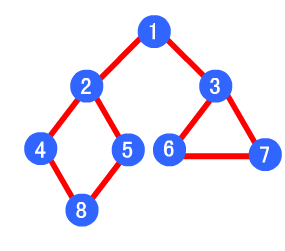
BFS类似于层序遍历，它的基本思想是：首先访问起始顶点v, 接着从v出发，依次访问各个未访问过的邻接顶点w1,w2....，然后再依次访问w1,w2...的所有未被访问过的邻接顶点。依次类推，直到图中所有的顶点都被访问过为止。如下例子：

图片来源：这里

bfs遍历的结果就是： 1->2->3->4->5->6->7->8

算法导论对bsf算法描述是这样的：

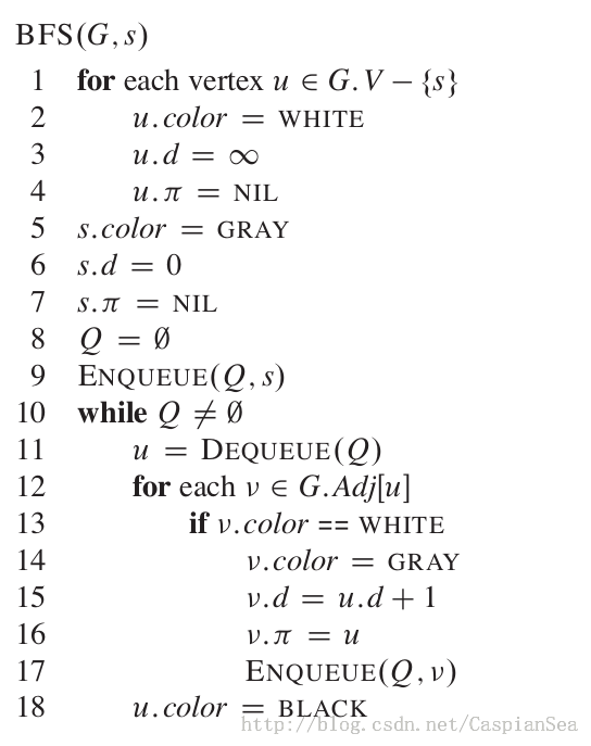
s.d 表示s到邻接结点的距离， s.π表示其前驱。
白色表示未访问过的结点，灰色表示发现了的结点，黑色表示已访问过的结点

算法描述：

1. 访问给定源结点v，并标记该点v已被访问
2. 将结点v进队
3. 当队列非空时，继续执行，否则算法结束
4. 出队，取队头结点u
5. 访问结点u的第一个邻接点w
6. 若w不存在，则转到第3步，若w存在则循环执行以下3步
   
   1. 结点w未被访问，将w标记为已访问
   2. 将结点w入队
   3. 查找结点u的继w邻接结点后的下一个邻接结点w，转到步骤6

这里我只放上bsf的关键代码

private void bfs(AdjecncyListGraph g, int s) {
        for(int v = 0; v < g.vNums(); v++) {
            distance[v] = Integer.MAX_VALUE;
        }
        LinkedList<Integer> queue = new LinkedList<Integer>();
        distance[s] = 0;
        marked[s] = true;
        queue.offer(s);
        while(!queue.isEmpty()) {
            int v = queue.poll();
            path.add(v);
            for(int w : g.getBags(v)) {
                if(!marked[w]) {
                    edgeTo[w] = v;
                    distance[w] = distance[v] + 1;
                    marked[w] = true;
                    queue.offer(w);
                }
            }
        }
    }

BFS需要一个辅助队列，n个顶点都要入队一次，空间复杂度为O(n)

当采用邻接表存储时，每个顶点都需要搜索一次，时间复杂度为O(n)。在搜索任一顶点时，每条边至少访问一次，时间复杂度为O(E)。因此总的时间复杂度为O(N + E)

当采用邻接矩阵存储时，查找每个邻接点的时间为O(N),因此时间复杂度为O(n^2)

深度优先搜索（Depth-First-Search,DFS）

DFS类似树的先序遍历。基本思想是：首先访问某个起始顶点v，然后从v出发，访问与v邻接且未被访问的任一顶点w1， 再访问与w1邻接且未被访问的任一顶点w2, ...重复上述过程。当不能再继续向下访问时，依次退回到最近被访问的顶点。若它还有其他的邻接点未被访问过，则从该点开始上面的过程。直到图中的所有点都被访问过为止。

图片来源： 这里

dfs遍历的结果就是： 1->2->4->8->5->3->6->7

算法描述：

1. 访问初始结点v，并标记结点v为已访问
2. 查找结点v的第一个邻接结点w
3. 若w存在，则继续执行4，否则算法结束
4. 若w未被访问，对w进行深度优先遍历递归（即把w当做另一个v，然后进行步骤123
5. 查找结点v的w邻接结点的下一个邻接结点，转到步骤3
   其实dfs就是一个递归过程

public void dfs(AdjecncyListGraph g, int v){
            marked[v]  = true;
            paths.add(v);
            for(int w : g.getBags(v)) {
                if(!marked[w]) {
                    edgeTo[w] = v;
                    marked[w] = true;
                    dfs(g, w);
                }
            }
    }

当采用邻接矩阵存储时，查找每个顶点的邻接点的时间为O(V),因此总的时间复杂度为O(V^2)

当采用邻接表存储时，查找每个顶点的邻接点的时间为O(E),访问顶点的时间复杂度为O(V),因此总的时间复杂度为O(V + E)

三、图的常见算法

1.最小生成树(Minimum-Spanning-Tree)

关于生成树：一个连通图的极小连通子图，它包含了图的所有顶点，并且只含尽可能少的边。这意味着对于生成树来说，若砍去它的一条边，就会使生成树变成非连通图，增加一条边就会出现环。

对于一个带权的无向图G, 生成树不同，每颗树的权也不一定相同。其中权值最小的那颗，即为最小生成树。

1. 最小生成树不是唯一的，即最小生成树的树形可能不同。当图G中的各边的权值互不相等时，它的最小生成树是唯一的。若无向连通图G的边比顶点数少1，即G本身就是一棵树，则最小生成树就是它本身。
2. 最小生成树的边权值之和是唯一的。
   下面给出一个MST的通用算法伪代码：

MST(G) {
    T = NULL;
    while T 未形成一颗生成树
        do 找到权值最小的边，并且该边加入T后不会产生回路
         T = T ∪ T‘
}

Prim算法

Prim算法是用来从带权图中搜索最小生成树的一种算法。
算法过程如下：

• 从单一顶点开始，普里姆算法按照以下步骤逐步扩大树中所含顶点的数目，直到遍及连通图的所有顶点。

• 输入：一个加权连通图，其中顶点集合为V，边集合为E；
  
  • 初始化：Vnew = {x}，其中x为集合V中的任一节点（起始点），Enew = {}；
  • 重复下列操作，直到Vnew = V：
  • 在集合E中选取权值最小的边（u, v），其中u为集合Vnew中的元素，而v则是V中没有加入Vnew的顶点（如果存在有多条满足前述条件即具有相同权值的边，则可任意选取其中之一）；
  • 将v加入集合Vnew中，将（u, v）加入集合Enew中；
    输出：使用集合Vnew和Enew来描述所得到的最小生成树。

算法伪代码：

Prim(G, T) {
    T = NULL;
    U = {w};    //添加任一顶点w
    while((V - U)!=NULL) {
        设(u, v)是u ∈ U 与 v ∈ （V - U),且权值最小的边
        T = T ∪ (u, v);
        U = U ∪ v ;
    }
}

Prim算法时间复杂度为O(V^2),比较适合于求稠密图的最小生成树。

Kruskal算法

Kruskal算法是一种按权值的递增次序选择合适的边来构成最小生成树的方法。

1. 新建图G，G中拥有原图中相同的节点，但没有边
2. 将原图中所有的边按权值从小到大排序
3. 从权值最小的边开始，如果这条边连接的两个节点于图G中不在同一个连通分量中，则添加这条边到图G中
4. 重复3，直至图G中所有的节点都在同一个连通分量中

算法伪代码：

 KRUSKAL-FUNCTION(G, w)
     F := 空集合
     for each 图 G 中的顶点 v
         do 將 v 加入森林 F
     所有的边(u, v) ∈ E依权重 w 递增排序
    for each 边(u, v) ∈ E
         do if u 和 v 不在同一棵子树
             then F := F ∪ {(u, v)}
                 將 u 和 v 所在的子树合并

2.最短路径