@wudawufanfan
2017-01-08T12:26:07.000000Z
字数 11220
阅读 1669
The final work-Quantum mechanics
Introduction
quantum mechanics, inscrutable and stupendous way of doing physics and yet, no-one knows why it works. I have always been amazed by the wonders of quantum world and always looked for the ways of grasping its significance. There are only a few problems in quantum mechanics that can be solved exactly, most notably the harmonic oscillator, a particle in the box, and the hydrogen atom.
Text
Time independent schrodinger equation
The time-independent schrodinger equation for a particle in three dimensions is
is Plank's constant, m is the mass of the particle, V is the potential energy, E is the energy of the particle, and is the wave function. When properly normalized, is the probability per unit volume that the partice will be found at .
An interesting property is that this eibenvalue problem in many cases solutions exist only for certain special discrete energy that can be solved analytically.
The simplest example is when potential is zero for free particle.
The Schrodinger equation then becomes
which has the general solution
which yeilds
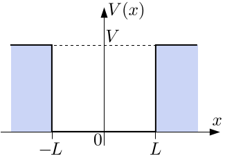
A more realistic situation is that the particle is confined to a box that extends from to . The potential is zero inside the box and infinite outsid the box called infinite square potential well.
For simplicity, we only discuss the direction of x.
and
Then we get a set of simple sinsoidal functions and cosine functions.
numerical method for time-independent Schrodinger equation in one dimension
Clearly, the Schrodinger equation is very similar in form to the equations of motion in connection with projectiles. Starting with initial values for and we were able to numerically intergrate forward with position to obtain. If is an even function of x, the wave functions can be written as purely even or purely odd functions of x. Thus, we can set initial condition as and or and .
At the same time, we can written the usual finite-difference form
For infinite well, the wave function must vanish at the walls. This is satisfied by certain energy.The thing is – this way we can get infinitely many solutions. But not all of them are meaningful. We need to find only those solutions where does not diverge at the edges of x. If it diverges, it disobeys the condition of square-integrability: and we deal with the physical falseness.
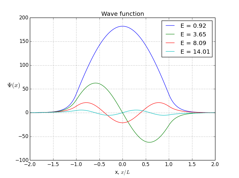
So here’s what we do: we run value of particle’s energy E from 0 to some value, say Vo, and calculate for each E. Value of (at the far outside of the finite well – where b>>L), is put into the separate list whose roots (places where it crosses zero) are to be found. Only those energies E for which is zero are taken in consideration and represent valid state of the particle. Here we see first of many weird things happening in the quantum world – particle can not have any value for kinetic energy, only some of discrete numbers.
def SE(psi, x):"""Returns derivatives for the 1D schrodinger eq.Requires global value E to be set somewhere. State0 isfirst derivative of the wave function psi, and state1 isits second derivative."""state0 = psi[1]state1 = 2.0*(V(x) - E)*psi[0]return array([state0, state1])
(Note: I’ve put m so that , just for simplicity). This function prepares state-space only. Following function does the real job, calls the state-space function and calculates the wave function for a given energy E. It also returns value of at the location x=b to test divergence.
def Wave_function(energy):"""Calculates wave function psi for the given valueof energy E and returns value at point b"""global psiglobal EE = energypsi = odeint(SE, psi0, x)return psi[-1,0]
Of course, for the first step there is no previous step – that’s why we introduce variable , which holds initial conditions: and
def find_all_zeroes(x,y):"""Gives all zeroes in y = f(x)"""all_zeroes = []s = sign(y)for i in range(len(y)-1):if s[i]+s[i+1] == 0:zero = brentq(Wave_function, x[i], x[i+1])all_zeroes.append(zero)return all_zeroes
Once we have the values of for a range of energies we need to distinguish those states where diverges. This is done using the Brent method to find a zero of the function f on the sign changing interval [a , b]. For an array of energies e we will check the sign of the . When the sign changes, it means that crosses zero point and now we can call brentq() to find the exact zero-point.
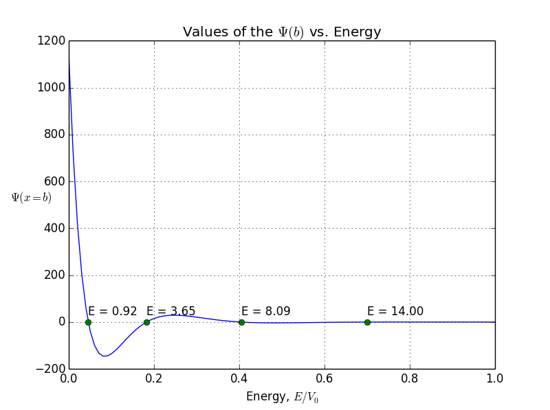
In this example, I put to 20(it looks like a finite well), L to 1, and m so that . We obtain only 4 four allowed bound states with energies 0.92, 3.65, 8.09, and 14.
A general potential well
For if we chose and we get something called symmetrical case, so left side is just mirrored right side. But if we reverse initial conditions so that and , we get antisymmetric case. Why is that so? I’ll tell you just that symmetrical states correspond to the cosine based functions, while antisymmetric correspond to the sine based functions. More about it will come a bit later.
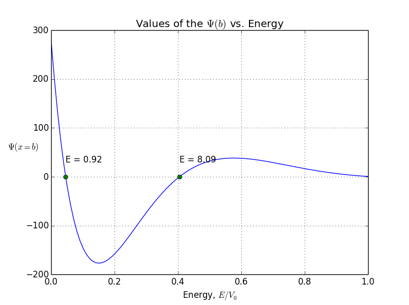
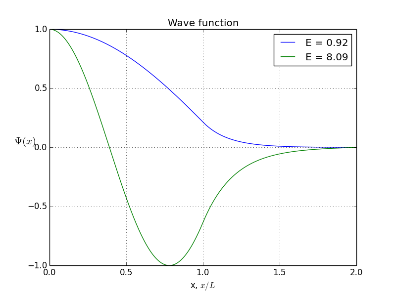
allowed energy and wave function for symmetrical states
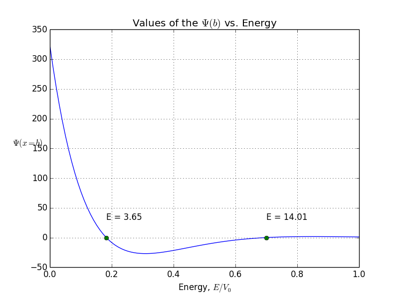

allowed energy and wave function for antisymmetrical states
You see, the odeint() requires the initial conditions at x = 0, assuming x goes from 0 to b. But what if I give it values -b < x< b? Normally, we expect to be o. But if we put initial conditions to be zero, we won’t get any non-zero result. That’s how the odeint() works, I can not prevent it. So here is where I cheat: I put x to be from -b to b, but initial conditions are not zero. Instead, they are some arbitrarily small value. Of course, odeint() will mess up values, but, interestingly, the shape of the function will stay correct!So, let’s do it again. Energies of allowed states are already calculated, it’s the first graph you see in this article. Bound states are here, presented in symmetrical and antisymmetrical case:
of course, I'm interesting in other figure's potential like a sphere.
In polar coordinates Schrödinger's equation reads:
Inside the well, where the potential is zero, would be set to zero.
Taking a as our length scale and as our energy scale, we gain the dimensionless form
we seek a solution
we find

and equation for is easy
Our "boundary condition" is that if we go round the origin exactly once, the value of the wavefunction is exactly the same, i.e., the wavefunction must be the same at and :
This leaves us with the r' differential equation. We will find it convenient to divide the above equation by E'-U0', but we will need to pay attention as to the sign of (E'-U0'). When (E'-U0')>0 we are in a classically allowed region, and we expect the wavefunction to oscillate with a wavelength that depends on the particle's momentum... sin(kr) like solutions are to be expected. When (E'-U0')<0 we are in a classically disallowed region, and we expect the wavefunction to exponentially decay...exp(-r) like solutions are to be expected. We'll handle both cases at the same time, sometimes by using ± signs where the top case (+ here) refers to a classically allowed region and the bottom case (- here) refers to a classically disallowed region. We substitute:
in our r' differential equation, producing a differential equation which I'll write in three equivalent forms:
The result is a little complx
As we expect that a second order linear differential equation should have two independent solutions, we're only half way there. is regular at =0, the other Bessel function: (also known as ) explodes at =0, and hence is not part of normalizable wavefunctions. Here are the basic large and small argument behaviors of and
As for show above, for large we expect oscillations like exp[±i]


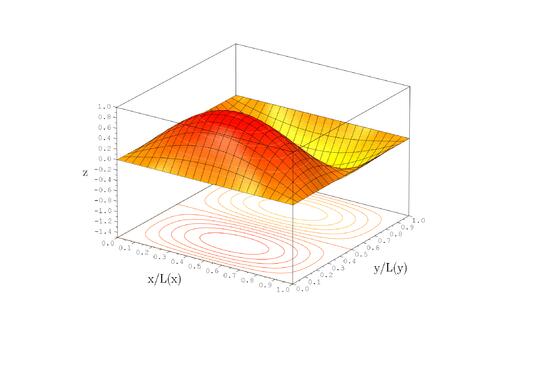
use matlab, I can figure out Bessel function in three diemension
a = 2*pi;[X Y] = meshgrid(-1:0.01:1,-1:0.01:1);R = sqrt(X.^2+Y.^2);f = (2*besselj(1,a*R(:))./R(:)).^2;mesh(X,Y,reshape(f,size(X)));axis vis3d;

Y and J are real functions and hence oscillate like sin and cos. If we want, we can put Y and J together to produce something that for large oscillates like exp[±i]. The results are called Hankel functions:

Here is the over all solution::
Because the angular dependence is "simple" we can usefully plot the wavefunction just as a function of r'. Here are "stacked wavefunction" plots for m=0,1,2:
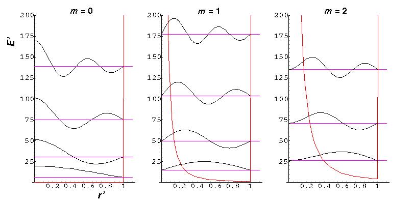
The red line is the classical "effective potential": (which is the "centrifugal potential") plus the infinite square well. Note that the centrifugal barrier excludes non-zero m wavefunctions from the origin.
| m, | root | E' |
|---|---|---|
| 0,0 | 2.4 | 5.78 |
| 1,0 | 3.8 | 14.68 |
| 2,0 | 5.1 | 26.37 |
| 0,1 | 5.5 | 30.47 |
| 3.0 | 6.4 | 40.71 |
| 1,1 | 7.0 | 49.22 |
Quantum tunneling
In classical physics, when a ball is rolled slowly up a large hill, it will come to a stop and roll back, because it doesn't have enough energy to get over the top of the hill to the other side. However, the Schrödinger equation predicts that there is a small probability that the ball will get to the other side of the hill, even if it has too little energy to reach the top. This is called quantum tunneling. It is related to the distribution of energy: although the ball's assumed position seems to be on one side of the hill, there is a chance of finding it on the other side.
distribution of wave function along x with time
Harmonic oscillator
The Schrodinger equation for the harmonic oscillator is
It is a notable quantum system to solve for; since the solutions are exact (but complicated – in terms of Hermite polynomials), and it can describe or at least approximate a wide variety of other systems, including vibrating atoms, molecules and atoms or ions in lattices and approximating other potentials near equilibrium points. It is also the basis of perturbation methods in quantum mechanics.
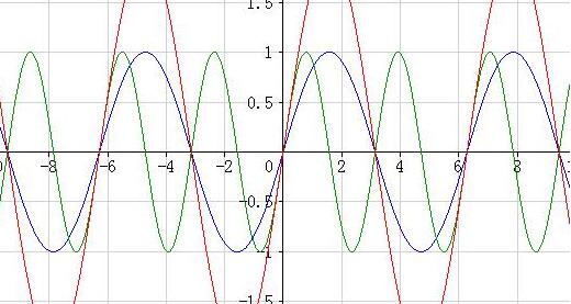
The analytic solutions are
we can see the solution for n=0 is the ground state which is a even function and the first exciting state for n=1 is a odd state which means the wave function is zero at x=0.
we can plot the harmonic oscillator mode and a set of figures to suit the possible solutions
A harmonic oscillator in classical mechanics (A–B) and quantum mechanics (C–H). In (A–B), a ball, attached to a spring, oscillates back and forth. (C–H) are six solutions to the Schrödinger Equation for this situation. The horizontal axis is position, the vertical axis is the real part (blue) or imaginary part (red) of the wavefunction. Stationary states, or energy eigenstates, which are solutions to the time-independent Schrödinger equation, are shown in C, D, E, F, but not G or H.E is the ground state and D is the first exciting state and so on.
The uncertainty principle
Schrödinger required that a wave packet solution near position r with wavevector near k will move along the trajectory determined by classical mechanics for times short enough for the spread in k (and hence in velocity) not to substantially increase the spread in r. Since, for a given spread in k, the spread in velocity is proportional to Planck's constant ħ, it is sometimes said that in the limit as ħ approaches zero, the equations of classical mechanics are restored from quantum mechanics.Great care is required in how that limit is taken, and in what cases.
When converge, will diverge,and vice versa.
use the analytic method for python, we can polt both of them at the same time
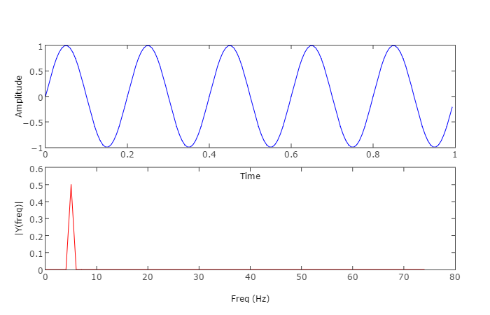
a interesting example is when wave function for x is
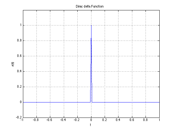
we can find the momentum distribution is equally everywhere.
of course, a general wave is Gauss wave packet like following.
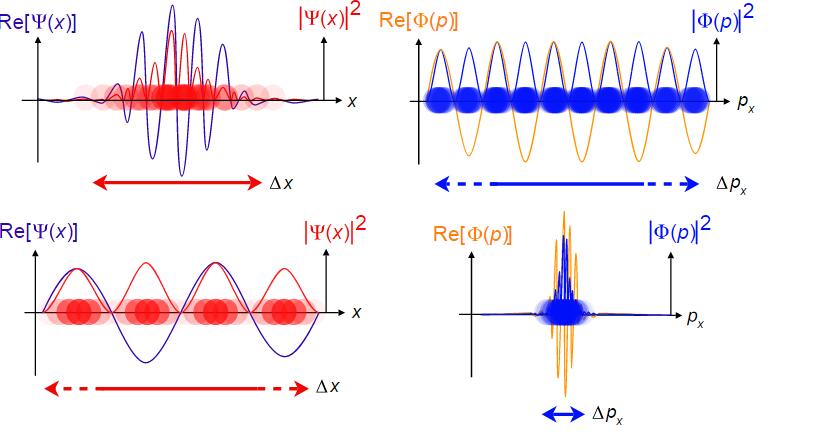
distribution of place and momentum
In physics, this is a famous principle called uncertainty principle which can be deduced by Schrödinger function.
which precisely show the relation between them.
Time-dependent Schrödinger
A wave function that satisfies the non-relativistic Schrödinger equation with V = 0. In other words, this corresponds to a particle traveling freely through empty space. The real part of the wave function is plotted here.
there are many interesting phenomenon in this problem, and I'll continue to do it.
codes
code1_find energy.py
code2_wave function along time.py
code3.py
code4_schord.py
code5_ bessel function
code6_fourier transform
code7_harmonic motion
