The numerical problem in the decays of two types of nucleus

calculation decay nucles

---

Introduction

A radioactive decay problem involving two types of nuclei,A and B,with populations $N_A(t)$ and $N_B(t)$.That the type A nuclei decay to form type B nuclei according to the differential equations

$$\frac{dN_A}{dN_B}=\frac{N_B}{\tau _B}-\frac{N_A}{\tau _A}$$
$$\frac{dN_B}{dt}=\frac{N_A}{\tau _A}-\frac{N_B}{\tau _B}$$
while $\tau _B=\tau _A$ for simplicity.
Now we should solve this system of equations for the numbers of nuclei,$N_A$ and $N_B$, as functions of time.

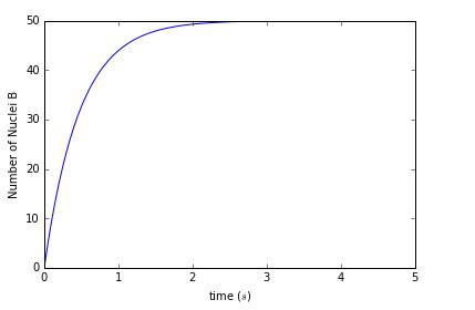
# -*- coding: utf-8 -*-
"""
Created on Sat Oct  1 14:44:46 2016
@author: 帆帆
"""
import pylab as pl
class uranium_decay:
    def __init__(self, number_of_nuclei_A = 100, number_of_nuclei_B=0, time_constant = 1, time_of_duration = 5, time_step = 0.05):
        # unit of time is second
        self.n_uranium_A = [number_of_nuclei_A]
        self.n_uranium_B = [number_of_nuclei_B]
        self.t = [0]
        self.tau = time_constant
        self.dt = time_step
        self.time = time_of_duration
        self.nsteps = int(time_of_duration // time_step + 1)
        print("Initial number of nuclei A ->", number_of_nuclei_A)
        print("Initial number of nuclei B->", number_of_nuclei_B)
        print("Time constant ->", time_constant)
        print("time step -> ", time_step)
        print("total time -> ", time_of_duration)
    def calculate(self):
        for i in range(self.nsteps):
            tmpA = self.n_uranium_A[i] + (self.n_uranium_B[i] / self.tau -self.n_uranium_A[i] / self.tau)* self.dt
            tmpB = self.n_uranium_B[i] + (self.n_uranium_A[i] / self.tau -self.n_uranium_B[i] / self.tau)* self.dt
            self.n_uranium_A.append(tmpA)
            self.n_uranium_B.append(tmpB)
            self.t.append(self.t[i] + self.dt)
    def show_results(self):
        pl.plot(self.t, self.n_uranium_A)
        pl.xlabel('time ($s$)')
        pl.ylabel('Number of Nuclei A')
        pl.show()
        pl.plot(self.t, self.n_uranium_B)
        pl.xlabel('time ($s$)')
        pl.ylabel('Number of Nuclei B')
        pl.show()
a = uranium_decay()
a.calculate()
a.show_results()

[the two results and the combination]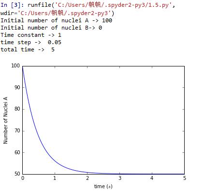

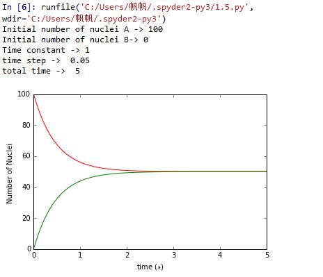
In attacking the radioactive decay problem we were led to treat time as a discrete variable.Such a discretization of time,or space,or both,is a common practice in numerical calculation,and brings up two related questions:

1. How do we konw that the errors introduced by this discretencess are negligible
2. How do we choose the value of such a step size for a calculation
   We know
   $\begin{cases} \frac{dN_A}{dN_B}=\frac{N_B}{\tau _B}-\frac{N_A}{\tau _A} \\ \frac{dN_B}{dt}=\frac{N_A}{\tau _A}-\frac{N_B}{\tau _B} \end{cases}$
   $\frac{d}{dt}$$\binom{N_A}{N_B}$=$\begin{pmatrix}-1&1\\1&-1\end{pmatrix}$$\binom{N_A}{N_B}$
   solve this first order differential equations with initial conditions we have
   $\begin{cases} N_A=50+50e^{-2t}\\N_B=50-50e^{-2t}\end {cases}$

import pylab as pl
class uranium_decay:
    def __init__(self, number_of_nuclei_A = 100, number_of_nuclei_B=0, time_constant = 1, time_of_duration = 5, time_step = 0.05):
        # unit of time is second
        self.n_uranium_A = [number_of_nuclei_A]
        self.n_uranium_B = [number_of_nuclei_B]
        self.t = [0]
        self.tau = time_constant
        self.dt = time_step
        self.time = time_of_duration
        self.nsteps = int(time_of_duration // time_step + 1)
        print("Initial number of nuclei A ->", number_of_nuclei_A)
        print("Initial number of nuclei B->", number_of_nuclei_B)
        print("Time constant ->", time_constant)
        print("time step -> ", time_step)
        print("total time -> ", time_of_duration)
    def calculate(self):
        for i in range(self.nsteps):
            tmpA = self.n_uranium_A[i] + (self.n_uranium_B[i] / self.tau -self.n_uranium_A[i] / self.tau)* self.dt
            tmpB = self.n_uranium_B[i] + (self.n_uranium_A[i] / self.tau -self.n_uranium_B[i] / self.tau)* self.dt
            self.n_uranium_A.append(tmpA)
            self.n_uranium_B.append(tmpB)
            self.t.append(self.t[i] + self.dt)
    def show_results(self):
        pl.plot(self.t, self.n_uranium_A,'r')
        pl.plot(self.t, self.n_uranium_B,'g',)
        pl.xlabel('time ($s$)')
        pl.ylabel('Number of Nuclei ')
        pl.show()
import math
class exact_results_check(uranium_decay):
    def show_results(self):
        self.etA = []
        self.etB = []
        for i in range(len(self.t)):
            tempA = 50+50*math.exp(- self.t[i] / self.tau)
            tempB = 50-50*math.exp(- self.t[i] / self.tau)
            self.etA.append(tempA)
            self.etB.append(tempB)
        pl.plot(self.t, self.etA)
        pl.plot(self.t, self.etB)
        pl.plot(self.t, self.n_uranium_A, '*')
        pl.plot(self.t, self.n_uranium_B, '*')
        pl.xlabel('time ($s$)')
        pl.ylabel('Number of Nuclei')
        pl.xlim(0, self.time)
        pl.show()        
a = exact_results_check()
a.calculate()
a.show_results()

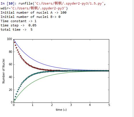
clearly,the simulation results is a bit different from the real result.

Improvement

import pylab as pl
class uranium_decay:
    def __init__(self, number_of_nuclei_A = 100, number_of_nuclei_B=0, time_constant = 1, time_of_duration = 5, time_step = 0.05):
        # unit of time is second
        self.n_uranium_A = [number_of_nuclei_A]
        self.n_uranium_B = [number_of_nuclei_B]
        self.t = [0]
        self.tau = time_constant
        self.dt = time_step
        self.time = time_of_duration
        self.nsteps = int(time_of_duration // time_step + 1)
        print("Initial number of nuclei A ->", number_of_nuclei_A)
        print("Initial number of nuclei B->", number_of_nuclei_B)
        print("Time constant ->", time_constant)
        print("time step -> ", time_step)
        print("total time -> ", time_of_duration)
    def calculate(self):
        for i in range(self.nsteps):
            tmpA = self.n_uranium_A[i] + (self.n_uranium_B[i] / self.tau -self.n_uranium_A[i] / self.tau)* self.dt
            tmpB = self.n_uranium_B[i] + (self.n_uranium_A[i] / self.tau -self.n_uranium_B[i] / self.tau)* self.dt
            self.n_uranium_A.append(tmpA)
            self.n_uranium_B.append(tmpB)
            self.t.append(self.t[i] + self.dt)
class diff_step_check(uranium_decay):
    def show_results(self, style = 'b'):
        pl.plot(self.t, self.n_uranium_A, style)
        pl.plot(self.t, self.n_uranium_B, style)
        pl.xlabel('time ($s$)')
        pl.ylabel('Number of Nuclei')
        pl.xlim(0, self.time)
from pylab import *
b = diff_step_check(number_of_nuclei_A=100,number_of_nuclei_B=0, time_constant=1,time_of_duration = 5, time_step = 0.05)
b.calculate()
b.show_results()
c = diff_step_check(number_of_nuclei_A=100,number_of_nuclei_B=0, time_constant=1,time_of_duration = 5, time_step = 0.0001)
c.calculate()
c.show_results('r')
show()

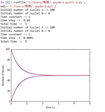
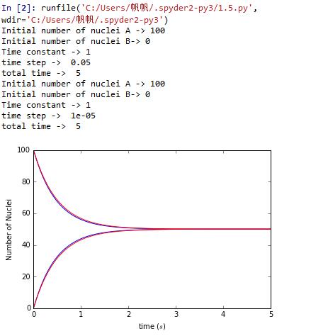
Change the time step didn't change the curve much.But we know this result is different from the real result a lot.So there may be another way to improve the accuracy of numerical results.

Conclusion

The numerical results are consistent with the idea that the system reaches a steady state in which $N_A$ and $N_B$ are constant.d$N_A$/dt and d$N_B$/dt vanish as well.

Thanks

Thanks for Caihao's PPT.