The billiard problem

未分类

Introduction

A ball moving without friction on a horizontal table and imagine that there are walls at the edges of the table that reflect the ball perfectly and that there is no frictional force between the ball and the table.The ball is given some initial velocity,and we are to calculate and understand the resulting trajectory.This is konwn as the stadium billiard problem.

Text

1、

Except for the collisions with the walls,the motion of the billiard is quite simple.Between collisions the velocity is constant so we have
$\frac{dx}{dt}=v_x$
$\frac{dy}{dt}=v_y$
and the Euler solution gives an exact description of the motion across the table.Now we tend to the calculation for the the collisions
$\vec{v}_{i,⊥}=(\vec{v}_i\cdot\widehat{n})\widehat{n}$
$\vec{v}_{i,||}=\vec{v}_i-\vec{v}_{i,⊥}$
Once we have the components of $\vec{v}_i$ we can reflect the billiard.A mirrorlike reflection reverses the perpendicular component of velocity,but leaves the parallel component unchanged.Hence,the velocity after reflection from the wall is
$\vec{v}_{f,⊥}=-v_{i,⊥}$
$\vec{v}_{i,||}=v_{i,||}$

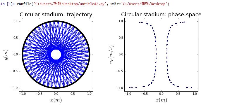
2、The trajectory of a billiard on a square table and the corresponding phase-space plots of $v_x$ versus x.

Firstly,consider a square table with a circular interior wall located in the center and a elliptical-bounded boundary.

from numpy import * 
import matplotlib.pyplot as plt
# class: BILLIARD solves for a stadium-shaped boundary
# where:
#        x0, y0, vx0, vy0: initial position of billiard 
#        dt, time : time step and total time
#        alpha: the length cube region 
class BILLIARD(object):
    def __init__(self,_alpha=0.,_r=1.,_x0=0.2,_y0=0.,_vx0=0.6,_vy0=0.8,_dt=0.001,_time=300):
        self.alpha, self.r, self.dt, self.time, self.n = _alpha, _r, _dt, _time, int(_time/_dt)
        self.x, self.y, self.vx, self.vy = [_x0], [_y0], [_vx0], [_vy0]
    def cal(self):            # use Euler method to solve billiard motion
        for i in range(self.n):
            self.nextx = self.x[-1]+self.vx[-1]*self.dt
            self.nexty = self.y[-1]+self.vy[-1]*self.dt
            self.nextvx, self.nextvy = self.vx[-1], self.vy[-1]
            if (self.nexty>self.alpha*self.r and self.nextx**2+(self.nexty-self.alpha*self.r)**2>self.r**2) \
                    or (self.nexty<-self.alpha*self.r and self.nextx**2+(self.nexty+self.alpha*self.r)**2>self.r**2) \
                    or (self.nextx>self.r) \
                    or (self.nextx<-self.r):
                self.nextx=self.x[-1]
                self.nexty=self.y[-1]
                while not( \
                        (self.nexty>self.alpha*self.r and self.nextx**2+(self.nexty-self.alpha*self.r)**2>self.r**2) \
                        or (self.nexty<-self.alpha*self.r and self.nextx**2+(self.nexty+self.alpha*self.r)**2>self.r**2) \
                        or (self.nextx>self.r) \
                        or (self.nextx<-self.r)):
                    self.nextx=self.nextx+self.nextvx*self.dt/100
                    self.nexty=self.nexty+self.nextvy*self.dt/100
                if self.nexty>self.alpha*self.r:
                    self.v = array([self.nextvx,self.nextvy])
                    self.norm =  1/self.r*array([self.nextx, self.nexty-self.alpha*self.r])
                    self.v_perpendicular = dot(self.v, self.norm)*self.norm
                    self.v_parrallel = self.v-self.v_perpendicular
                    self.v_perpendicular= -self.v_perpendicular
                    self.nextvx, self.nextvy= (self.v_parrallel+self.v_perpendicular)[0],(self.v_parrallel+self.v_perpendicular)[1]
                elif self.nexty<-self.alpha*self.r:
                    self.v = array([self.nextvx,self.nextvy])
                    self.norm =  1/self.r*array([self.nextx, self.nexty+self.alpha*self.r])
                    self.v_perpendicular = dot(self.v, self.norm)*self.norm
                    self.v_parrallel = self.v-self.v_perpendicular
                    self.v_perpendicular= -self.v_perpendicular
                    self.nextvx, self.nextvy= (self.v_parrallel+self.v_perpendicular)[0],(self.v_parrallel+self.v_perpendicular)[1]
                else:
                    self.nextvx, self.nextvy= -self.nextvx, self.nextvy
            self.x.append(self.nextx)
            self.y.append(self.nexty)
            self.vx.append(self.nextvx)
            self.vy.append(self.nextvy)
    def plot_position(self,_ax):        # give trajectory plot
        _ax.plot(self.x,self.y,'-b',label=r'$\alpha=$'+'  %.2f'%self.alpha)
        _ax.plot([self.r]*10,linspace(-self.alpha*self.r,self.alpha*self.r,10),'-k',lw=5)
        _ax.plot([-self.r]*10,linspace(-self.alpha*self.r,self.alpha*self.r,10),'-k',lw=5)
        _ax.plot(self.r*cos(linspace(0,pi,100)),self.r*sin(linspace(0,pi,100))+self.alpha*self.r,'-k',lw=5)
        _ax.plot(self.r*cos(linspace(pi,2*pi,100)),self.r*sin(linspace(pi,2*pi,100))-self.alpha*self.r,'-k',lw=5)
    def plot_phase(self,_ax,_secy=0):        # give phase-space plot
        self.secy=_secy
        self.phase_x, self.phase_vx = [], []
        for i in range(len(self.x)):
            if abs(self.y[i]-self.secy)<1E-3 :
                self.phase_x.append(self.x[i])
                self.phase_vx.append(self.vx[i])
        _ax.plot(self.phase_x,self.phase_vx,'ob',markersize=2,label=r'$\alpha=$'+'  %.2f'%self.alpha)
# give a trajectory and phase space plot          
fig= plt.figure(figsize=(10,10))
ax1=plt.axes([0.1,0.55,0.35,0.35])
ax2=plt.axes([0.6,0.55,0.35,0.35])
ax3=plt.axes([0.1,0.1,0.35,0.35])
ax4=plt.axes([0.6,0.1,0.35,0.35])
ax1.set_xlim(-1.1,1.1)
ax2.set_xlim(-1.1,1.1)
ax3.set_xlim(-1.1,1.1)
ax4.set_xlim(-1.1,1.1)
ax1.set_ylim(-1.1,1.1)
ax2.set_ylim(-1.1,1.1)
ax3.set_ylim(-1.1,1.1)
ax4.set_ylim(-1.1,1.1)
ax1.set_xlabel(r'$x (m)$',fontsize=18)
ax1.set_ylabel(r'$y (m)$',fontsize=18)
ax1.set_title('Circular stadium: trajectory',fontsize=18)
ax2.set_xlabel(r'$x (m)$',fontsize=18)
ax2.set_ylabel(r'$v_x (m/s)$',fontsize=18)
ax2.set_title('Circular stadium: phase-space',fontsize=18)
ax3.set_xlabel(r'$x (m)$',fontsize=18)
ax3.set_ylabel(r'$y (m)$',fontsize=18)
ax3.set_title('Billiard'+r'$\alpha=0.05$'+': trajectory',fontsize=18)
ax4.set_xlabel(r'$x (m)$',fontsize=18)
ax4.set_ylabel(r'$v_x (m/s)$',fontsize=18)
ax4.set_title('Billiard '+r'$\alpha=0.05$'+': phase-space',fontsize=18)
cmp=BILLIARD()
cmp.cal()
cmp.plot_position(ax1)
cmp.plot_phase(ax2)
cmp=BILLIARD(0.05)
cmp.cal()
cmp.plot_position(ax3)
cmp.plot_phase(ax4)
plt.show()

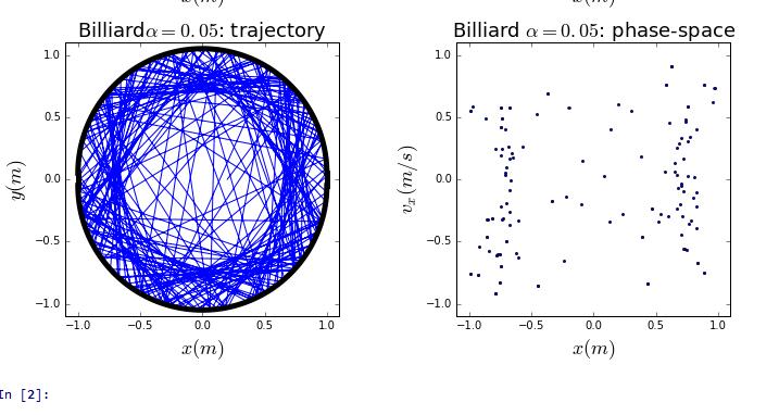
from numpy import * 
import matplotlib.pyplot as plt
# class: BILLIARD solves for a elliptical-bounded boundary
# where:
#        x0, y0, vx0, vy0: initial position of billiard 
#        dt, time : time step and total time
class BILLIARD(object):
    def __init__(self,_x0=sqrt(2),_y0=0.,_vx0=0,_vy0=1,_dt=0.001,_time=500):
        self.dt, self.time, self.n = _dt, _time, int(_time/_dt)
        self.x, self.y, self.vx, self.vy = [_x0], [_y0], [_vx0], [_vy0]
    def cal(self):            # use Euler method to solve billiard motion
        for i in range(self.n):
            self.nextx = self.x[-1]+self.vx[-1]*self.dt
            self.nexty = self.y[-1]+self.vy[-1]*self.dt
            self.nextvx, self.nextvy = self.vx[-1], self.vy[-1]
            if self.nextx**2/3+self.nexty**2>1:
                self.nextx=self.x[-1]
                self.nexty=self.y[-1]
                while not(self.nextx**2/3+self.nexty**2>1):
                    self.nextx=self.nextx+self.nextvx*self.dt/100
                    self.nexty=self.nexty+self.nextvy*self.dt/100
                self.norm=array([self.nextx,3*self.nexty])
                self.norm=self.norm/sqrt(dot(self.norm,self.norm))
                self.v=array([self.nextvx,self.nextvy])
                self.v_perpendicular=dot(self.v,self.norm)*self.norm
                self.v_parrallel=self.v-self.v_perpendicular
                self.v_perpendicular=-self.v_perpendicular
                [self.nextvx,self.nextvy]=self.v_parrallel+self.v_perpendicular
            self.x.append(self.nextx)
            self.y.append(self.nexty)
            self.vx.append(self.nextvx)
            self.vy.append(self.nextvy)
    def plot_position(self,_ax):        # give trajectory plot
        _ax.plot(self.x,self.y,'-b',label='Ellipse'+r'$a=2,b=1$')
        _ax.plot(sqrt(3)*cos(linspace(0,2*pi,200)),sin(linspace(0,2*pi,200)),'-k',lw=5)
    def plot_phase(self,_ax,_secy=0):        # give phase-space plot
        self.secy=_secy
        self.phase_x, self.phase_vx = [], []
        for i in range(len(self.x)):
            if abs(self.y[i]-self.secy)<1E-3 and abs(self.vx[i])<0.95:
                self.phase_x.append(self.x[i])
                self.phase_vx.append(self.vx[i])
        _ax.plot(self.phase_x,self.phase_vx,'ob',markersize=2,label='Ellipse'+r'$a=2,b=1$')
# give a trajectory and phase space plot        
fig= plt.figure(figsize=(10,4))
ax1=plt.axes([0.1,0.15,0.35,0.7])
ax2=plt.axes([0.6,0.15,0.35,0.7])
ax1.set_xlim(-2,2)
ax1.set_ylim(-1.1,1.1)
ax2.set_xlim(-2,2)
ax2.set_ylim(-1.1,1.1)  
ax1.set_title('Elliptical boundary: '+r'$a^2 =3,b^2 = 1$',fontsize=18)
ax2.set_title('Phase-space: '+r'$a^2 =3,b^2 = 1$',fontsize=18)
ax1.set_xlabel(r'$x(m)$',fontsize=18)
ax1.set_ylabel(r'$y(m)$',fontsize=18)
ax2.set_xlabel(r'$x(m)$',fontsize=18)
ax2.set_ylabel(r'$v_x (m/s)$',fontsize=18)
cmp=BILLIARD()
cmp.cal()
cmp.plot_position(ax1)
cmp.plot_phase(ax2)
plt.show()

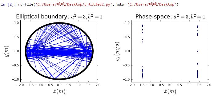
if the shape of boundary is line,the the code for python is easy without losing generalizability.The only one need to calculate is the tranformation of velocity.Here we set four boundaries are
y$\le$$\frac{5}{4}$(x+3)
y$\le$-$\frac{5}{4}$(x-3)
y$\le$2.5
y$\ge$0。
When x$\ge$0, we only need to use the boundaries y$\le$-$\frac{5}{4}$(x-3) and y$\le$2.5
When the particle reach the boundary $\le$-$\frac{5}{4}$(x-3),
line y=-$\frac{5}{4}$(x-3)'s normal unit vector is $\vec{n}$=(cos$\theta$,sin$\theta$), while tan$\theta$=$\frac{4}{5}$
$\vec{v}_{i,⊥}$=$(v_x$i+$v_y$j)•(cos$\theta$i+sin$\theta$j)(cos$\theta$,sin$\theta$)
The line's direction unit vector is (cos$\varphi$,sin$\varphi$), while tan$\varphi$=-$\frac{5}{4}$
$\vec{v}_{i,//}$=($v_x$i+$v_y$j)•(cos$\varphi$i+sin$\varphi$j)(cos$\varphi$,sin$\varphi$)
so the velocity after colision is $\vec{v}_{i,//}-\vec{v}_{i,⊥}$
$\vec{v}=[v_x(cos^2\varphi-sin^2\theta)+v_y(sin\varphi cos\varphi-sin\theta cos\theta)]i+[v_x(cos\varphi sin\varphi$-$cos\theta sin\theta)+v_y(sin^2\varphi-sin^2\theta)]j$

import numpy as np
from pylab import *
x=[0]
y=[1]
vx,vy=2.3,3
time,i,dt=0,0,0.001
sdt=0.00001
velocity=[4]
while time<=300:
    X=x[i]+vx*dt
    Y=y[i]+vy*dt
    if Y>0 and Y<2.5:
        if X>=0:
            if Y<-X*4.0/3.0+4:
                x.append(X)
                y.append(Y)
                velocity.append(vx)
            else:
                x1=x[i]+vx*sdt
                y1=y[i]+vy*sdt
                if y1<-x1*4.0/3.0+4:
                    x.append(x1)
                    y.append(y1)
                    velocity.append(vx)
                else:
                    char1=-vx*(9.0/41.0)-vy*(40.0/41.0)         
                    char2=-vx*(40.0/41.0)+vy*(9.0/41.0)
                    vx=char1
                    vy=char2                
                    x.append(x[i]+vx*sdt)
                    y.append(y[i]+vy*sdt)
                    velocity.append(vx)
        if X<0:
            if Y<X*4.0/3.0+4:
                x.append(X)
                y.append(Y)
                velocity.append(vx)
            else:
                x2=x[i]+vx*sdt
                y2=y[i]+vy*sdt
                if y2<x2*4.0/3.0+4:
                    x.append(x2)
                    y.append(y2)
                    velocity.append(vx)
                else:
                    char3=-vx*(9/41)+vy*(40/41)
                    char4=vx*(40/41)+vy*(9/41)
                    vx=char3
                    vy=char4
                    x.append(x[i]+vx*sdt)
                    y.append(y[i]+vy*sdt)
                    velocity.append(vx)
    if Y>=2.5:
        x4=x[i]+vx*sdt
        y4=y[i]+vy*sdt
        if y4<2.5:
            x.append(x4)
            y.append(y4)
            velocity.append(vx)
        else:   
            vy=-vy
            x.append(x[i]+vx*sdt)
            y.append(y[i]+vy*sdt)
            velocity.append(vx)
    if Y<=0:
        x3=x[i]+vx*sdt
        y3=y[i]+vy*sdt
        if y3>0:
            x.append(x3)
            y.append(y3)
            velocity.append(vx)
        else:   
            vy=-vy
            x.append(x[i]+vx*sdt)
            y.append(y[i]+vy*sdt)
            velocity.append(vx)
    time=time+dt
    i=i+1
plt.figure(figsize=(16,5.5))
subplot(1,2,1)
plt.title("vx0=2.3,vy0=3")
plt.xlabel("x")
plt.ylabel("y")
plt.xticks([-3,-2,-1,0,1,2,3])
plt.yticks([0,1,2,3,4])
plt.xlim(-3,3)
plt.ylim(0,4)
plt.plot([1.125,3],[2.5,0],color="blue",label="isosceles triangle",linewidth=2)
plt.plot([-1.125,1.125],[2.5,2.5],color="blue",linewidth=2)
plt.plot([-3,-1.125],[0,2.5],color="blue",linewidth=2)
plt.plot([-3,3],[0,0],color="blue",linewidth=2)
plt.plot(x,y,label="trajectory",color="red")
plt.scatter(0,1,color="black",alpha=1,linewidth=4,label="initial")
plt.legend()
subplot(1,2,2)
plt.xlabel("x")
plt.ylabel("vx")
for i in range(1000):
    if 1000*i<=len(x):
        plt.scatter(x[1000*i],velocity[1000*i])
plt.show()

We can change the velocity to get different trajectory in which some is chaoic

the velocity is vx=0,vy=2

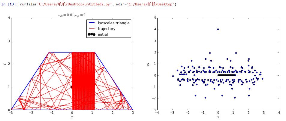
the velocity is vx=0.01,vy=2

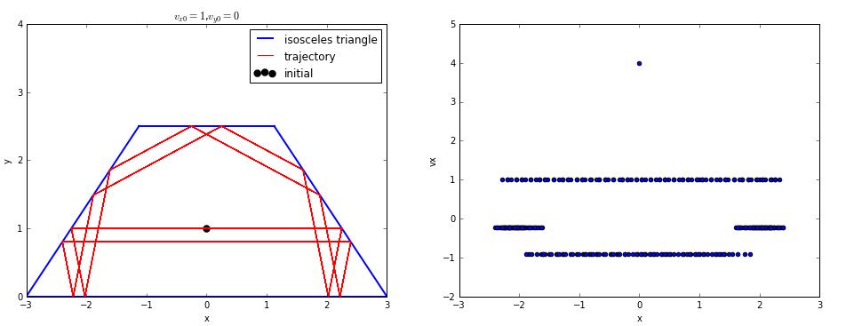
the velocity is vx=1,vy=0

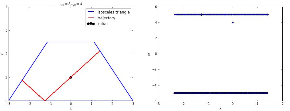
the velocity is vx=5,vy=4

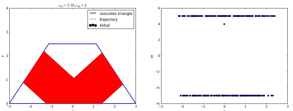
the velocity is vx=5.01,vy=4
we can see a small change to initial condition may cause big difference to trajectory.

Conclusion

For any realistically shaped container,such motion is likely to be chaotic and thus unpredictable.

Thanks

cheng yaoyang's code.
wu yuqiao's vpython.