Potentials and Fields

electric potential and fields:laplace's equation

In regions of space that do not contain any electric charges,the electric potential obeys Laplace's equation
$\frac{\partial^2V}{\partial x^2}+\frac{\partial^2V}{\partial y^2}+\frac{\partial^2V}{\partial z^2}=0$
Our problem is to find the function V(x,y,z) that satisfies both Laplace's equation and the specified boundary conditions.
As usual we discretize the independent variables,in the case x,y and z.Points in our space are then specified by integers i,j,k.Our goal is to determine the potential $V(i,j,k)=V(i\triangle x,j\triangle y,k\triangle z)$ on this lattice of points.
$\frac{\partial^2V}{\partial x^2}=\frac{V(i+1,j,k)+V(i-1,j,k)-2V(i,j+1,k)}{(\triangle x)^2}$
is we set $(\triangle x)^2=(\triangle y)^2=(\triangle z)^2$
Inserting them all into Laplace's equation and solving for V(i,j,k) we find
$V(i,j,k)=\frac{1}{6}[V(i+1,j,k)+V(i-1,j,k)+$
$V(i,j+1,k)+V(i,j-1,k)+V(i,j,k+1)+V(i,j,k-1)]$

$V_0(i,j,k)\xrightarrow{Eq}V_1(i,j,k)\xrightarrow{Eq}V_2(i,j,k)\xrightarrow{Eq}$
FIGURE:Schematic flowchart for the relaxation algorithm

the problem of calculating the electric potential inside the square box

the boundary conditions we assume that the face of the box at x=-1 is held at V=-1,while V=+1 on the face at x=1. and V(i,j,k) is independent of k.
$V(i,j,k)=\frac{1}{4}[V(i+1,j,k)+V(i-1,j,k)+V(i,j+1,k)$
$+V(i,j-1,k)]$

Jacobi Method (via wikipedia):

An algorithm for determining the solutions of a diagonally dominant system of linear equations. Each diagonal element is solved for, and an approximate value is plugged in. The process is then iterated until it converges. This algorithm is a stripped-down version of the Jacobi transformation method of matrix diagonalization.
In other words, Jacobi’s method is an iterative method for solving systems of linear equations, very similar to Gauss-Seidel Method. Beginning with the standard Ax = b, where A is a known matrix and b is a known vector we can use Jacobi’s method to approximate/solve x. The one caveat being the A matrix must be diagonally dominant to ensure that the method converges, although it occasionally converges without this condition being met.

import numpy as np
from scipy.linalg import solve
def jacobi(A, b, x, n):
    D = np.diag(A)
    R = A - np.diagflat(D)
    for i in range(n):
        x = (b - np.dot(R,x))/ D
    return x
'''___Main___'''
A = np.array([[4.0, -2.0, 1.0], [1.0, -3.0, 2.0], [-1.0, 2.0, 6.0]])
b = [1.0, 2.0, 3.0]
x = [1.0, 1.0, 1.0]
n = 25
x = jacobi(A, b, x, n)
print (solve(A, b))
init [1.0, 1.0, 1.0]
000 [ 0.5         0.33333333  0.33333333]
001 [ 0.33333333 -0.27777778  0.47222222]
002 [-0.00694444 -0.24074074  0.64814815]
003 [-0.03240741 -0.23688272  0.57908951]
004 [-0.01321373 -0.29140947  0.57355967]
005 [-0.03909465 -0.28869813  0.5949342 ]
006 [-0.04308262 -0.28307542  0.58971694]
007 [-0.03896694 -0.28788291  0.58717804]
008 [-0.04073597 -0.28820362  0.58946648]
009 [-0.04146843 -0.28726767  0.58927855]
010 [-0.04095347 -0.28763711  0.58884448]
011 [-0.04102968 -0.28775483  0.58905346]
012 [-0.04114078 -0.28764092  0.58908   ]
013 [-0.04109046 -0.28766026  0.58902351]
014 [-0.04108601 -0.28768115  0.58903834]
015 [-0.04110016 -0.28766977  0.58904605]
016 [-0.0410964  -0.28766935  0.5890399 ]
017 [-0.04109465 -0.2876722   0.58904039]
018 [-0.0410962  -0.28767129  0.58904162]
019 [-0.04109605 -0.28767098  0.58904107]
020 [-0.04109576 -0.28767131  0.58904099]
021 [-0.0410959  -0.28767126  0.58904114]
022 [-0.04109592 -0.2876712   0.5890411 ]
023 [-0.04109588 -0.28767124  0.58904108]
024 [-0.04109589 -0.28767124  0.5890411 ]
Sol  [-0.04109589 -0.28767124  0.5890411 ]
Act  [-0.04109589 -0.28767123  0.5890411 ]

Now we consider two complicated cases where an analytic solution is difficult.
A long infinitely long,hollow prism,with metallic walls and a square cross-section.The prism and inner conductor are presumed to be infinite in extent along z,The inner conductor is held at V=1 and the walls of the prism at V=0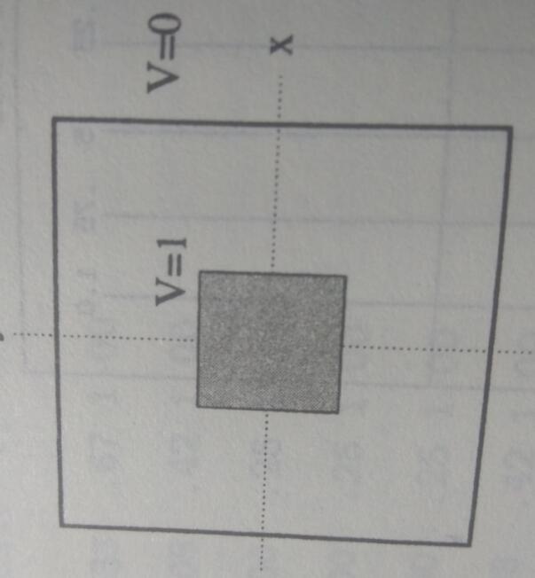

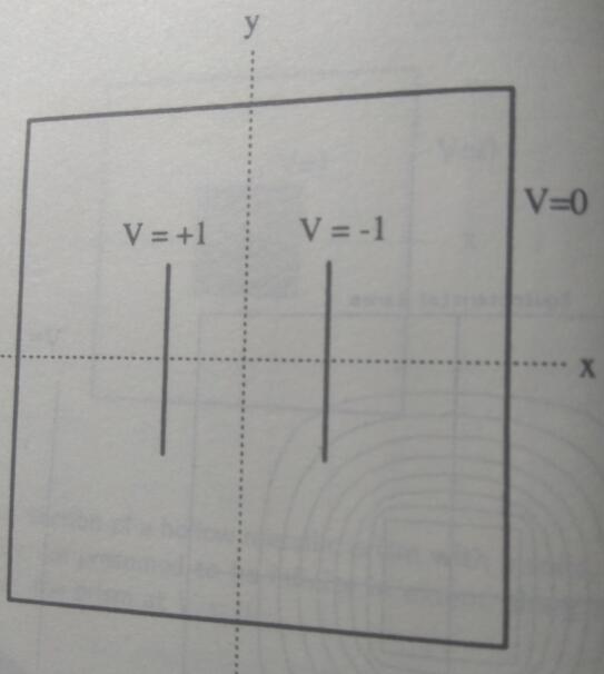
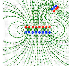
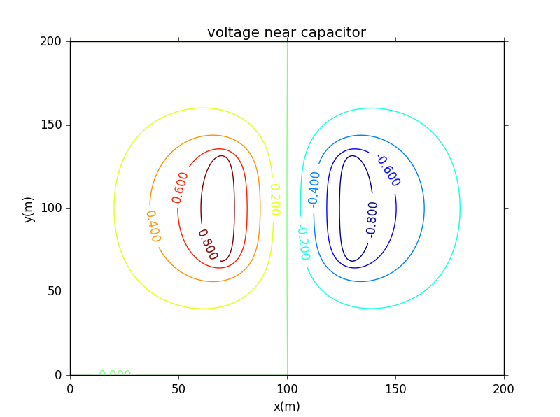
Another example is two capacitor plates held at V=1(left plate) and V=-1(right plate).The square boundary surrounding the plates is held at V=0

from numpy import *
import mpl_toolkits.mplot3d
import matplotlib.pyplot as plt
from matplotlib import cm
from matplotlib.ticker import LinearLocator, FormatStrFormatter
'''
class Electric_Field
this class solves the potential euation of capacitor
where: 
              V1: potential of the left plate
              V2: potential of the right palte
              n: size of one side
'''
class ELECTRIC_FIELD(object):
    def __init__(self, V1=1, V2=-1, V_boundary=0, n=30):
        self.V1=float(V1)
        self.V2=float(V2)
        self.V_boundary=float(V_boundary)
        self.n=int(n)
        self.s1, self.s3=int(n/3), int(n/3)
        self.s2, self.s4=int(self.n-2-2*self.s1), int(self.n-2*self.s3)
        self.V=[]
        for j in range(self.n):
            self.V.append([0.0]*self.n)
        for j in [0,self.n-1]:
            self.V[j]=[self.V_boundary]*self.n
        for j in range(self.s3,self.s3+self.s4):
            self.V[j][self.s1]=self.V1
            self.V[j][self.s1+self.s2+1]=self.V2            
    def update_V_SOR(self):       # use SOR method solve the potential
        self.alpha=2./(1.+pi/self.n)
        self.counter=0
        while True:
            self.delta_V=0.
            for j in range(1,self.n-1):
                for i in range(1,self.n-1):
                    if (j in range(self.s3,self.s3+self.s4)) and (i in [self.s1,self.s1+self.s2+1]):
                        continue
                    self.next_V=1./4.*(self.V[j-1][i]+self.V[j+1][i]+self.V[j][i-1]+self.V[j][i+1])
                    self.V[j][i]=self.alpha*(self.next_V-self.V[j][i])+self.V[j][i]
                    self.delta_V=self.delta_V+abs(self.alpha*(self.next_V-self.V[j][i]))
            self.counter=self.counter+1
            if (self.delta_V < abs(self.V2-self.V1)*(1.0E-5)*self.n*self.n and self.counter >= 10):
                break
        print ('itertion length n=',self.n,'  ',self.counter,' times')
    def Ele_field(self,x1,x2,y1,y2):    # calculate the Electirc field  
        self.dx=abs(x1-x2)/float(self.n-1)
        self.Ex=[]
        self.Ey=[]
        for j in range(self.n):
            self.Ex.append([0.0]*self.n)
            self.Ey.append([0.0]*self.n)
        for j in range(1,self.n-1,1):
            for i in range(1,self.n-1,1):
                self.Ex[j][i]=-(self.V[j][i+1]-self.V[j][i-1])/(2*self.dx)
                self.Ey[j][i]=-(self.V[j-1][i]-self.V[j+1][i])/(2*self.dx)
    def plot_3d(self,ax,x1,x2,y1,y2):   # give 3d plot the potential
        self.x=linspace(x1,x2,self.n)
        self.y=linspace(y2,y1,self.n)
        self.x,self.y=meshgrid(self.x,self.y)
        self.surf=ax.plot_surface(self.x,self.y,self.V, rstride=1, cstride=1, cmap=cm.coolwarm)
        ax.set_xlim(x1,x2)
        ax.set_ylim(y1,y2)
        ax.zaxis.set_major_locator(LinearLocator(10))
        ax.zaxis.set_major_formatter(FormatStrFormatter('%.01f'))
        ax.set_xlabel('x (m)',fontsize=14)
        ax.set_ylabel('y (m)',fontsize=14)
        ax.set_zlabel('Electric potential (V)',fontsize=14)
        ax.set_title('Potential near capacitor',fontsize=18)
    def plot_2d(self,ax1,ax2,x1,x2,y1,y2):    # give 2d plot of potential and electric field
        self.x=linspace(x1,x2,self.n)
        self.y=linspace(y2,y1,self.n)
        self.x,self.y=meshgrid(self.x,self.y)
        cs=ax1.contour(self.x,self.y,self.V)
        plt.clabel(cs, inline=1, fontsize=10)
        ax1.set_title('Equipotential lines',fontsize=18)
        ax1.set_xlabel('x (m)',fontsize=14)
        ax1.set_ylabel('y (m)',fontsize=14)
        for j in range(1,self.n-1,1):
            for i in range(1,self.n-1,1):
                ax2.arrow(self.x[j][i],self.y[j][i],self.Ex[j][i]/40,self.Ey[j][i]/40,fc='k', ec='k')             
        ax2.set_xlim(-1.,1.)
        ax2.set_ylim(-1.,1.)
        ax2.set_title('Electric field',fontsize=18)
        ax2.set_xlabel('x (m)',fontsize=14)
        ax2.set_ylabel('y (m)',fontsize=14)
    def export_data(self,x1,x2,y1,y2):
        self.mfile=open(r'd:\data.txt','w')
        self.x=linspace(x1,x2,self.n)
        self.y=linspace(y2,y1,self.n)
        self.x,self.y=meshgrid(self.x,self.y)
        for j in range(self.n):
            for i in range(self.n):
                print >> self.mfile, self.x[j][i],self.y[j][i],self.V[j][i]
        self.mfile.close()
# give plot of potential and electric field 
fig=plt.figure(figsize=(10,5))
ax1=plt.axes([0.1,0.1,0.35,0.8])
ax2=plt.axes([0.55,0.1,0.35,0.8])
cmp=ELECTRIC_FIELD(1,-1,0,20)
cmp.update_V_SOR()
cmp.Ele_field(-1,1,-1,1)
cmp.plot_2d(ax1,ax2,-1.,1.,-1.,1.)
plt.show()     
# give 3d plot of potential
fig=plt.figure(figsize=(14,7))
ax1= plt.subplot(1,2,1,projection='3d')
cmp=ELECTRIC_FIELD()
cmp.update_V_SOR()
cmp.plot_3d(ax1,-1.,1.,-1.,1.)
fig.colorbar(cmp.surf, shrink=0.5, aspect=5)
ax2= plt.subplot(1,2,2,projection='3d')
cmp=ELECTRIC_FIELD(5,-0.5,0,20)
cmp.update_V_SOR()
cmp.plot_3d(ax2,-1.,1.,-1.,1.)
fig.colorbar(cmp.surf, shrink=0.5, aspect=5)
plt.show(fig)

from __future__ import division
import matplotlib
import numpy as np
import matplotlib.cm as cm
import matplotlib.mlab as mlab
import matplotlib.pyplot as plt
from mpl_toolkits.mplot3d import Axes3D
# initialize the grid
grid = []
for i in range(201):    
    row_i = []
    for j in range(201):
        if i == 0 or i == 200 or j == 0 or j == 200:
            voltage = 0
        elif 70<=i<=130 and j == 70:
            voltage = 1
        elif 70<=i<=130 and j == 130:
            voltage = -1
        else:
            voltage = 0
        row_i.append(voltage)
    grid.append(row_i)
# define the update_V function (Gauss-Seidel method)
def update_V(grid):
    delta_V = 0
    for i in range(201):    
        for j in range(201):
            if i == 0 or i == 200 or j == 0 or j == 200:
                pass
            elif 70<=i<=130 and j == 70:
                pass
            elif 70<=i<=130 and j == 130:
                pass
            else:
                voltage_new = (grid[i+1][j]+grid[i-1][j]+grid[i][j+1]+grid[i][j-1])/4
                voltage_old = grid[i][j]
                delta_V += abs(voltage_new - voltage_old)
                grid[i][j] = voltage_new
    return grid, delta_V
# define the Laplace_calculate function
def Laplace_calculate(grid):
    epsilon = 10**(-5)*200**2
    grid_init = grid
    delta_V = 0
    N_iter = 0
    while delta_V >= epsilon or N_iter <= 10:
        grid_impr, delta_V = update_V(grid_init)
        grid_new, delta_V = update_V(grid_impr)
        grid_init = grid_new
        N_iter += 1
    return grid_new
matplotlib.rcParams['xtick.direction'] = 'out'
matplotlib.rcParams['ytick.direction'] = 'out'
x = np.linspace(0,200,201)
y = np.linspace(0,200,201)
X, Y = np.meshgrid(x, y)
Z = Laplace_calculate(grid)
plt.figure()
CS = plt.contour(X,Y,Z,10)
plt.clabel(CS, inline=1, fontsize=12)
plt.title('voltage near capacitor')
plt.xlabel('x(m)')
plt.ylabel('y(m)')
fig = plt.figure()
ax = fig.add_subplot(111, projection='3d')
ax.plot_surface(X, Y, Z)
ax.set_xlabel('x(m)')
ax.set_ylabel('y(m)')
ax.set_zlabel('voltage(V)')
ax.set_title('voltage distribution')
plt.show()

Mathematically the Jacobi method can be expressed as
$V_{new}(i,j)=\frac{1}{4}[V_{old}(i+1,j)+V_{old}(i-1,j)+V_{old}(i,j+1)+$
$V_{old}(i,j-1)]$
the simple improvement is the Gasuss-Seidel method.
$V_{new}(i,j)=\frac{1}{4}[V_{old}(i+1,j)+V_{new}(i-1,j)+V_{old}(i,j+1)+$
$V_{new}(i,j-1)]$
and we can think of $\triangle V(i,j)=V^*(i,j)-V_{old}(i,j)$
to speed up convergence we will change potential by a larger amount calculated according to
$V_{mew}(i,j)=\alpha\triangle V(i,j)+V_{old}(i,j)$
where $\alpha$ is a factor that measures how much we "over-relax"

from numpy import *
import mpl_toolkits.mplot3d
import matplotlib.pyplot as plt
from matplotlib import cm
from matplotlib.ticker import LinearLocator, FormatStrFormatter
import time
'''
class Electric_Field
this class solves the potential euation of capacitor
where: 
              V1: potential of the left plate
              V2: potential of the right palte
              n: size of one side
'''
class ELECTRIC_FIELD(object):
    def __init__(self, V1=1, V2=-1, V_boundary=0, n=30):
        self.V1=float(V1)
        self.V2=float(V2)
        self.V_boundary=float(V_boundary)
        self.n=int(n)
        self.s1, self.s3=int(n/3), int(n/3)
        self.s2, self.s4=int(self.n-2-2*self.s1), int(self.n-2*self.s3)
        self.V=[]
        for j in range(self.n):
            self.V.append([0.0]*self.n)
        for j in [0,self.n-1]:
            self.V[j]=[self.V_boundary]*self.n
        for j in range(self.s3,self.s3+self.s4):
            self.V[j][self.s1]=self.V1
            self.V[j][self.s1+self.s2+1]=self.V2            
    def update_V_Jacobi(self):
        self.counter=0                         # use Jacobi method solve the potential       
        while True:
            self.V_next=[]
            for j in range(self.n):
                self.V_next.append([0.0]*self.n)
            for j in range(self.n):
                for i in range(self.n):
                    self.V_next[j][i]=self.V[j][i]
            self.delta_V=0.
            for j in range(1,self.n-1):
                for i in range(1,self.n-1):
                    if (j in range(self.s3,self.s3+self.s4)) and (i in [self.s1,self.s1+self.s2+1]):
                        continue
                    self.V_next[j][i]=1./4.*(self.V[j-1][i]+self.V[j+1][i]+self.V[j][i-1]+self.V[j][i+1])
                    self.delta_V=self.delta_V+abs(self.V_next[j][i]-self.V[j][i])
            self.counter=self.counter+1
            for j in range(self.n):
                for i in range(self.n):
                    self.V[j][i]=self.V_next[j][i]
            if (self.delta_V < abs(self.V2-self.V1)*(1.0E-5)*self.n*self.n and self.counter >= 10):
                break
        print ('jacobi itertion length n=',self.n,'  ',self.counter,' times')
        return self.counter
    def update_V_Gauss(self):              # use Gauss-Seidel method solve the potential
        self.counter=0
        while True:
            self.delta_V=0.
            for j in range(1,self.n-1):
                for i in range(1,self.n-1):
                    if (j in range(self.s3,self.s3+self.s4)) and (i in [self.s1,self.s1+self.s2+1]):
                        continue
                    self.next_V=1./4.*(self.V[j-1][i]+self.V[j+1][i]+self.V[j][i-1]+self.V[j][i+1])
                    self.delta_V=self.delta_V+abs(self.next_V-self.V[j][i])
                    self.V[j][i]=self.next_V   
            self.counter=self.counter+1
            if (self.delta_V < abs(self.V2-self.V1)*(1.0E-5)*self.n*self.n and self.counter >= 10):
                break
        print ('gauss itertion length n=',self.n,'  ',self.counter,' times')
        return self.counter    
    def update_V_SOR(self):           # use SOR method solve the potential
        self.alpha=2./(1.+pi/self.n)
        self.counter=0
        while True:
            self.delta_V=0.
            for j in range(1,self.n-1):
                for i in range(1,self.n-1):
                    if (j in range(self.s3,self.s3+self.s4)) and (i in [self.s1,self.s1+self.s2+1]):
                        continue
                    self.next_V=1./4.*(self.V[j-1][i]+self.V[j+1][i]+self.V[j][i-1]+self.V[j][i+1])
                    self.V[j][i]=self.alpha*(self.next_V-self.V[j][i])+self.V[j][i]
                    self.delta_V=self.delta_V+abs(self.alpha*(self.next_V-self.V[j][i]))
            self.counter=self.counter+1
            if (self.delta_V < abs(self.V2-self.V1)*(1.0E-5)*self.n*self.n and self.counter >= 10):
                break
        print( 'SOR itertion length n=',self.n,'  ',self.counter,' times')
        return self.counter
    def Ele_field(self,x1,x2,y1,y2):       # calculate the Electirc field  
        self.dx=abs(x1-x2)/float(self.n-1)
        self.Ex=[]
        self.Ey=[]
        for j in range(self.n):
            self.Ex.append([0.0]*self.n)
            self.Ey.append([0.0]*self.n)
        for j in range(1,self.n-1,1):
            for i in range(1,self.n-1,1):
                self.Ex[j][i]=-(self.V[j][i+1]-self.V[j][i-1])/(2*self.dx)
                self.Ey[j][i]=-(self.V[j-1][i]-self.V[j+1][i])/(2*self.dx)
    def plot_3d(self,ax,x1,x2,y1,y2):       # give 3d plot the potential
        self.x=linspace(x1,x2,self.n)
        self.y=linspace(y2,y1,self.n)
        self.x,self.y=meshgrid(self.x,self.y)
        self.surf=ax.plot_surface(self.x,self.y,self.V, rstride=1, cstride=1, cmap=cm.coolwarm)
        ax.set_xlim(x1,x2)
        ax.set_ylim(y1,y2)
        ax.zaxis.set_major_locator(LinearLocator(10))
        ax.zaxis.set_major_formatter(FormatStrFormatter('%.01f'))
        ax.set_xlabel('x (m)',fontsize=14)
        ax.set_ylabel('y (m)',fontsize=14)
        ax.set_zlabel('Electric potential (V)',fontsize=14)
        ax.set_title('Potential near capacitor',fontsize=18)
    def plot_2d(self,ax1,ax2,x1,x2,y1,y2):     # give 2d plot of potential and electric field
        self.x=linspace(x1,x2,self.n)
        self.y=linspace(y2,y1,self.n)
        self.x,self.y=meshgrid(self.x,self.y)
        cs=ax1.contour(self.x,self.y,self.V)
        plt.clabel(cs, inline=1, fontsize=10)
        ax1.set_title('Equipotential lines',fontsize=18)
        ax1.set_xlabel('x (m)',fontsize=14)
        ax1.set_ylabel('y (m)',fontsize=14)
        for j in range(1,self.n-1,1):
            for i in range(1,self.n-1,1):
                ax2.arrow(self.x[j][i],self.y[j][i],self.Ex[j][i]/40,self.Ey[j][i]/40,fc='k', ec='k')             
        ax2.set_xlim(-1.,1.)
        ax2.set_ylim(-1.,1.)
        ax2.set_title('Electric field',fontsize=18)
        ax2.set_xlabel('x (m)',fontsize=14)
        ax2.set_ylabel('y (m)',fontsize=14)
    def export_data(self,x1,x2,y1,y2):          # export data
        self.mfile=open(r'd:\data.txt','w')
        self.x=linspace(x1,x2,self.n)
        self.y=linspace(y2,y1,self.n)
        self.x,self.y=meshgrid(self.x,self.y)
        for j in range(self.n):
            for i in range(self.n):
                print >> self.mfile, self.x[j][i],self.y[j][i],self.V[j][i]
        self.mfile.close()
#  compare three method   
n_min=10        # Jacobi method
n_max=50
n_jacobi=[]
iters_jacobi=[]
time_jacobi=[]
for i in range(n_min,n_max,2):
    start=time.clock()
    cmp=ELECTRIC_FIELD(1,-1,0,i)
    iters_jacobi.append(cmp.update_V_Jacobi())
    end=time.clock()
    time_jacobi.append(end-start)   
    n_jacobi.append(i)
n_gauss=[]         # Gauss Seidel method
iters_gauss=[]
time_gauss=[]
for i in range(n_min,n_max,2):
    start=time.clock()
    cmp=ELECTRIC_FIELD(1,-1,0,i)
    iters_gauss.append(cmp.update_V_Gauss())
    end=time.clock()
    time_gauss.append(end-start)   
    n_gauss.append(i)
n_SOR=[]       # SOR method
iters_SOR=[]
time_SOR=[]
for i in range(n_min,n_max,2):
    start=time.clock()
    cmp=ELECTRIC_FIELD(1,-1,0,i)
    iters_SOR.append(cmp.update_V_SOR())
    end=time.clock()
    time_SOR.append(end-start)
    n_SOR.append(i)
print( time_SOR)
#  export data
mfile=open(r'd:\data.txt','w')
for i in range(len(n_jacobi)):
    print ( n_jacobi[i], time_jacobi[i], time_gauss[i], time_SOR[i],file=mfile)
mfile.close()
# give a simple plot
fig=plt.figure(figsize=(14,7))
ax1=plt.axes([0.1,0.1,0.35,0.8])
ax2=plt.axes([0.55,0.1,0.35,0.8])
ax1.plot(n_jacobi,iters_jacobi,'or',markersize=5)
ax1.plot(n_gauss,iters_gauss,'ob',markersize=5)
ax1.plot(n_SOR,iters_SOR,'oy',markersize=5)
ax2.plot(n_jacobi,time_jacobi,'or',markersize=5)
ax2.plot(n_gauss,time_gauss,'ob',markersize=5)
ax2.plot(n_SOR,time_SOR,'oy',markersize=5)
plt.show(fig)

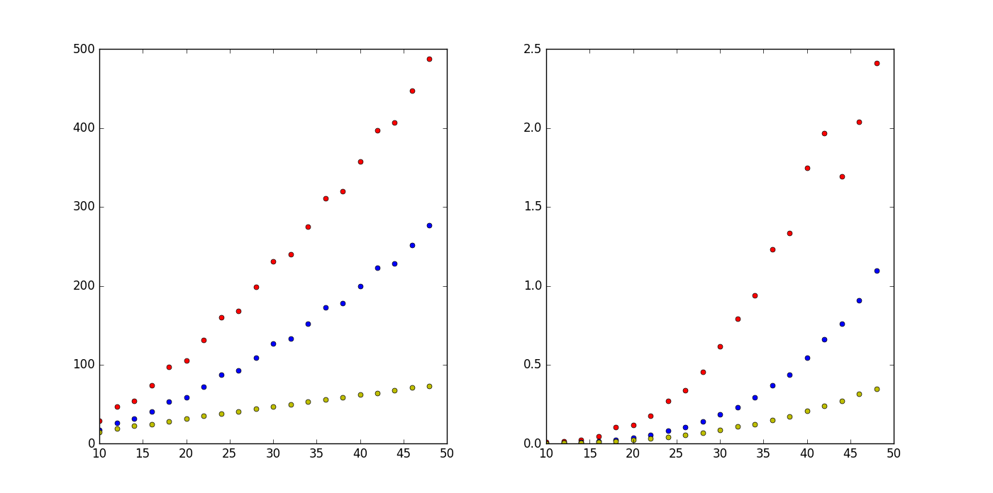
the relation of side length and number of interations(left) time
consuming(right)

$\begin{cases} red 　for 　Jacobi\\ blue　 for 　Gauss-Seidel 　method\\ yellow 　for 　simultaneous 　over-relaxation(SOR)\end{cases}$

from numpy import *
import mpl_toolkits.mplot3d
import matplotlib.pyplot as plt
from matplotlib import cm
from matplotlib.ticker import LinearLocator, FormatStrFormatter
import time
'''
class Electric_Field
this class solves the potential euation of capacitor
where: 
              V1: potential of the left plate
              V2: potential of the right palte
              n: size of one side
'''
class ELECTRIC_FIELD(object):
    def __init__(self, V1=1, V2=-1, V_boundary=0, n=30):
        self.V1=float(V1)
        self.V2=float(V2)
        self.V_boundary=float(V_boundary)
        self.n=int(n)
        self.s1, self.s3=int(n/3), int(n/3)
        self.s2, self.s4=int(self.n-2-2*self.s1), int(self.n-2*self.s3)
        self.V=[]
        for j in range(self.n):
            self.V.append([0.0]*self.n)
        for j in [0,self.n-1]:
            self.V[j]=[self.V_boundary]*self.n
        for j in range(self.s3,self.s3+self.s4):
            self.V[j][self.s1]=self.V1
            self.V[j][self.s1+self.s2+1]=self.V2              
    def update_V_SOR(self,alpha):       # use SOR method solve the potential
        self.alpha=float(alpha)
        self.counter=0
        while True:
            self.delta_V=0.
            for j in range(1,self.n-1):
                for i in range(1,self.n-1):
                    if (j in range(self.s3,self.s3+self.s4)) and (i in [self.s1,self.s1+self.s2+1]):
                        continue
                    self.next_V=1./4.*(self.V[j-1][i]+self.V[j+1][i]+self.V[j][i-1]+self.V[j][i+1])
                    self.delta_V=self.delta_V+abs(self.alpha*(self.next_V-self.V[j][i]))
                    self.V[j][i]=self.alpha*(self.next_V-self.V[j][i])+self.V[j][i]
            self.counter=self.counter+1
            if (self.delta_V < abs(self.V2-self.V1)*(1.0E-5)*self.n*self.n and self.counter >= 10):
                break
        print ('SOR itertion alpha= ',self.alpha,'  ',self.counter,' times')
        return self.counter
    def Ele_field(self,x1,x2,y1,y2):    # calculate the Electirc field  
        self.dx=abs(x1-x2)/float(self.n-1)
        self.Ex=[]
        self.Ey=[]
        for j in range(self.n):
            self.Ex.append([0.0]*self.n)
            self.Ey.append([0.0]*self.n)
        for j in range(1,self.n-1,1):
            for i in range(1,self.n-1,1):
                self.Ex[j][i]=-(self.V[j][i+1]-self.V[j][i-1])/(2*self.dx)
                self.Ey[j][i]=-(self.V[j-1][i]-self.V[j+1][i])/(2*self.dx)
    def plot_3d(self,ax,x1,x2,y1,y2):   # give 3d plot the potential
        self.x=linspace(x1,x2,self.n)
        self.y=linspace(y2,y1,self.n)
        self.x,self.y=meshgrid(self.x,self.y)
        self.surf=ax.plot_surface(self.x,self.y,self.V, rstride=1, cstride=1, cmap=cm.coolwarm)
        ax.set_xlim(x1,x2)
        ax.set_ylim(y1,y2)
        ax.zaxis.set_major_locator(LinearLocator(10))
        ax.zaxis.set_major_formatter(FormatStrFormatter('%.01f'))
        ax.set_xlabel('x (m)',fontsize=14)
        ax.set_ylabel('y (m)',fontsize=14)
        ax.set_zlabel('Electric potential (V)',fontsize=14)
        ax.set_title('Potential near capacitor',fontsize=18)
    def plot_2d(self,ax1,ax2,x1,x2,y1,y2):    # give 2d plot of potential and electric field
        self.x=linspace(x1,x2,self.n)
        self.y=linspace(y2,y1,self.n)
        self.x,self.y=meshgrid(self.x,self.y)
        cs=ax1.contour(self.x,self.y,self.V)
        plt.clabel(cs, inline=1, fontsize=10)
        ax1.set_title('Equipotential lines',fontsize=18)
        ax1.set_xlabel('x (m)',fontsize=14)
        ax1.set_ylabel('y (m)',fontsize=14)
        for j in range(1,self.n-1,1):
            for i in range(1,self.n-1,1):
                ax2.arrow(self.x[j][i],self.y[j][i],self.Ex[j][i]/40,self.Ey[j][i]/40,fc='k', ec='k')             
        ax2.set_xlim(-1.,1.)
        ax2.set_ylim(-1.,1.)
        ax2.set_title('Electric field',fontsize=18)
        ax2.set_xlabel('x (m)',fontsize=14)
        ax2.set_ylabel('y (m)',fontsize=14)
    def export_data(self,x1,x2,y1,y2):
        self.mfile=open(r'd:\data.txt','w')
        self.x=linspace(x1,x2,self.n)
        self.y=linspace(y2,y1,self.n)
        self.x,self.y=meshgrid(self.x,self.y)
        for j in range(self.n):
            for i in range(self.n):
                print >> self.mfile, self.x[j][i],self.y[j][i],self.V[j][i]
        self.mfile.close()
# change alpha and determine the number of iterations        
iters=[]
alpha=[]
for j in linspace(0.19,0.9,30):
    cmp=ELECTRIC_FIELD()
    alpha.append(j)
    iters.append(cmp.update_V_SOR(j))
for j in linspace(0.91,1.3,20):
    cmp=ELECTRIC_FIELD()
    alpha.append(j)
    iters.append(cmp.update_V_SOR(j))
for j in linspace(1.3,1.79,30):
    cmp=ELECTRIC_FIELD()
    alpha.append(j)
    iters.append(cmp.update_V_SOR(j))
for j in linspace(1.8,1.98,30):
    cmp=ELECTRIC_FIELD()
    alpha.append(j)
    iters.append(cmp.update_V_SOR(j))
mfile=open(r'd:\data.txt','w')
for i in range(len(alpha)):
    print(alpha[i],iters[i],file=mfile)
mfile.close()
fig=plt.figure(figsize=(8,8))
ax1=plt.subplot(111)
ax1.plot(alpha,iters,'ob')
ax1.set_xlabel('alpha')
ax1.set_ylabel('number of iterations')
plt.show(fig)

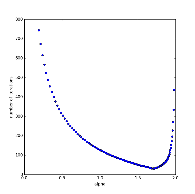
the relation between alpha and number of interations
we can find when $\alpha$ is around 1.5 to 2,we need the least work.

Thanks

Wu yuqiao and chengyaoyang's codes
Computational physics by Nicholas J.Giordano,Hisao Nakanishi