chapter3.18、3.19、3.20、3.21

未分类

This homework is about the problem of period doubling.

A show of vPython

this is the code for simulation

from __future__ import division
from visual import *
from math import *
# add some constants
q=0.5
l=9.8
g=9.8
f=2/3
dt=0.04
theta0=0.2
omega0=0
# add three ceilings
ceil1=box(pos=(-20,5,0),size=(5,0.5,2),material=materials.bricks)
ceil2=box(pos=(0,5,0),size=(5,0.5,2),material=materials.bricks)
ceil3=box(pos=(20,5,0),size=(5,0.5,2),material=materials.bricks)
ball1=sphere(pos=(-20+l*sin(theta0),5-l*cos(theta0),0),radius=1,material=materials.emissive,color=color.red)
ball2=sphere(pos=(l*sin(theta0),5-l*cos(theta0),0),radius=1,material=materials.emissive,color=color.yellow)
ball3=sphere(pos=(20+l*sin(theta0),5-l*cos(theta0),0),radius=1,material=materials.emissive,color=color.green)
ball1.omega=omega0
ball2.omega=omega0
ball3.omega=omega0
ball1.theta=theta0
ball2.theta=theta0
ball3.theta=theta0
ball1.t=0
ball2.t=0
ball3.t=0
ball1.F=0
ball2.F=0.5
ball3.F=1.2
string1=curve(pos=[ceil1.pos,ball1.pos],color=color.red)
string2=curve(pos=[ceil2.pos,ball2.pos],color=color.yellow)
string3=curve(pos=[ceil3.pos,ball3.pos],color=color.green)
po1=arrow(pos=ball1.pos,axis=(10*ball1.omega*cos(ball1.theta),10*ball1.omega*sin(ball1.theta),0),color=color.red)
po2=arrow(pos=ball2.pos,axis=(10*ball2.omega*cos(ball2.theta),10*ball2.omega*sin(ball2.theta),0),color=color.yellow)
po3=arrow(pos=ball3.pos,axis=(10*ball3.omega*cos(ball3.theta),10*ball3.omega*sin(ball3.theta),0),color=color.green)
while True:
    rate(100)
    ball1.omega=ball1.omega-((g/l)*sin(ball1.theta)+q*ball1.omega-ball1.F*sin(f*ball1.t))*dt
    ball2.omega=ball2.omega-((g/l)*sin(ball2.theta)+q*ball2.omega-ball2.F*sin(f*ball2.t))*dt
    ball3.omega=ball3.omega-((g/l)*sin(ball3.theta)+q*ball3.omega-ball3.F*sin(f*ball3.t))*dt
    angle1_new=ball1.theta+ball1.omega*dt
    while angle1_new>pi:
        angle1_new-=2*pi
    while angle1_new<-pi:
        angle1_new+=2*pi
    angle2_new=ball2.theta+ball2.omega*dt
    while angle2_new>pi:
        angle2_new-=2*pi
    while angle2_new<-pi:
        angle2_new+=2*pi
    angle3_new=ball3.theta+ball3.omega*dt
    while angle3_new>pi:
        angle3_new-=2*pi
    while angle3_new<-pi:
        angle3_new+=2*pi
    ball1.theta=angle1_new
    ball2.theta=angle2_new
    ball3.theta=angle3_new
    ball1.pos=(-20+l*sin(ball1.theta),5-l*cos(ball1.theta),0)
    ball2.pos=(l*sin(ball2.theta),5-l*cos(ball2.theta),0)
    ball3.pos=(20+l*sin(ball3.theta),5-l*cos(ball3.theta),0)
    string1.pos=[ceil1.pos,ball1.pos]
    string2.pos=[ceil2.pos,ball2.pos]
    string3.pos=[ceil3.pos,ball3.pos]
    po1.pos=ball1.pos
    po2.pos=ball2.pos
    po3.pos=ball3.pos
    po1.axis=(10*ball1.omega*cos(ball1.theta),10*ball1.omega*sin(ball1.theta),0)
    po2.axis=(10*ball2.omega*cos(ball2.theta),10*ball2.omega*sin(ball2.theta),0)
    po3.axis=(10*ball3.omega*cos(ball3.theta),10*ball3.omega*sin(ball3.theta),0)
    ball1.t=ball1.t+dt
    ball2.t=ball2.t+dt
    ball3.t=ball3.t+dt

TEXT

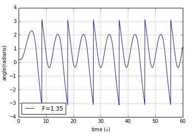
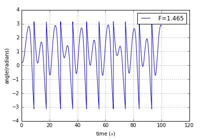
We use the same condition but different driving force
$F_D=1.35　　　　F_D=1.44　　　　F_D=1.465$

import math
import pylab as pl
class harmonic:
    def __init__(self, w_0 = 0, theta_0=0.2,  time_of_duration =60, time_step = 0.04,g=9.8,length=9.8,q=1/2,F=1.35,D=2/3):
        # unit of time is second
        self.n_uranium_A = [w_0]
        self.n_uranium_B = [theta_0]
        self.t = [0]
        self.g=g
        self.length=length
        self.dt = time_step
        self.time = time_of_duration
        self.nsteps = int(time_of_duration // time_step + 1)
        self.q=q
        self.F=F
        self.D=D
    def calculate(self):
        for i in range(self.nsteps):
            tmpA = self.n_uranium_A[i] -((self.g/self.length)*math.sin(self.n_uranium_B[i])+self.q*self.n_uranium_A[i]-self.F*math.sin(self.D*self.t[i]))*self.dt
            tmpB = self.n_uranium_B[i] + self.n_uranium_A[i]*self.dt
            self.n_uranium_A.append(tmpA)
            self.n_uranium_B.append(tmpB)
            self.t.append(self.t[i] + self.dt)
            if self.n_uranium_B[i+1]<-math.pi:
                self.n_uranium_B[i+1]=self.n_uranium_B[i+1]+2*math.pi
            if self.n_uranium_B[i+1]>math.pi:
                self.n_uranium_B[i+1]=self.n_uranium_B[i+1]-2*math.pi
            else:
                pass
    def show_results(self):
        pl.plot(self.t, self.n_uranium_B,label=' F=1.35')
        pl.xlabel('time ($s$)')
        pl.ylabel('angle(radians)')
        pl.legend(loc='best',frameon = True)
        pl.grid(True)
a = harmonic()
a.calculate()
a.show_results()

we find that the period is T,2T,4T



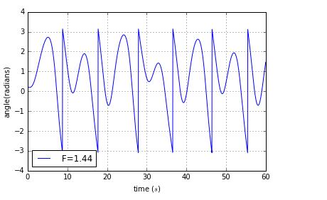
this picture is not good
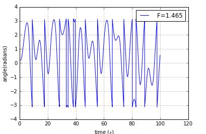
when we change the time step form 0.04 to 0.01,it tends to good reult

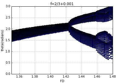
But if the period keeps on doubling,what about the transition to chaos?Our textbook give a way to appreciate how this transition comes about is with what is known as a bifurcation diagram.

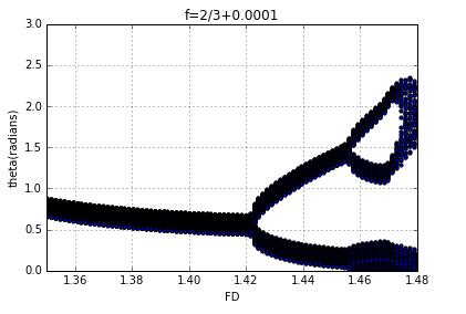
from __future__ import division
from math import *
from pylab import *
from numpy import *
# define a function that given amplitude of force, gives angle,avelo and t
def change_amp(F,f):
    # define some constants
    q = 0.5
    l = 9.8
    g = 9.8
    dt = pi/100
    theta0 = 0.2
    omega0 = 0
    angle = [theta0]
    avelo = [omega0]
    t = [0]
    an=[]
    # move the pendulum
    while t[-1] <= 1200*pi:
        avelo_new = avelo[-1] - ((g/l)*sin(angle[-1]) + q*avelo[-1] - F*sin(f*t[-1]))*dt
        avelo.append(avelo_new)
        angle_new = angle[-1] + avelo[-1]*dt
        while angle_new > pi:
            angle_new -= 2*pi
        while angle_new < -pi:
            angle_new += 2*pi
        angle.append(angle_new)
        if t[-1]>=900*pi:
            if t[-1]%(3*pi)<=dt:
                an.append(angle_new)
        t_new = t[-1] + dt
        t.append(t_new)
    return an
###
fdd_1=list(linspace(1.35,1.5,100))
fd_1=[]
th_1=[]
for i in fdd_1:
    points=change_amp(i,2/3)
    for j in points:
        fd_1.append(i)
        th_1.append(j)
###
###
scatter(fd_1,th_1,s=10)
grid(True)
xlim(1.35,1.48)
ylim(0,3)
title('f=2/3')
xlabel('FD')
ylabel('theta(radians)')
show()

we have get the bifurcation diagram when the frenquency is 2/3

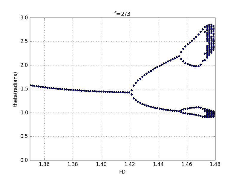
use the magnified plot of the diagram,we could estimate the point
at which the transition to period-$2^n$ behaviors take place.



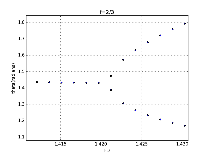
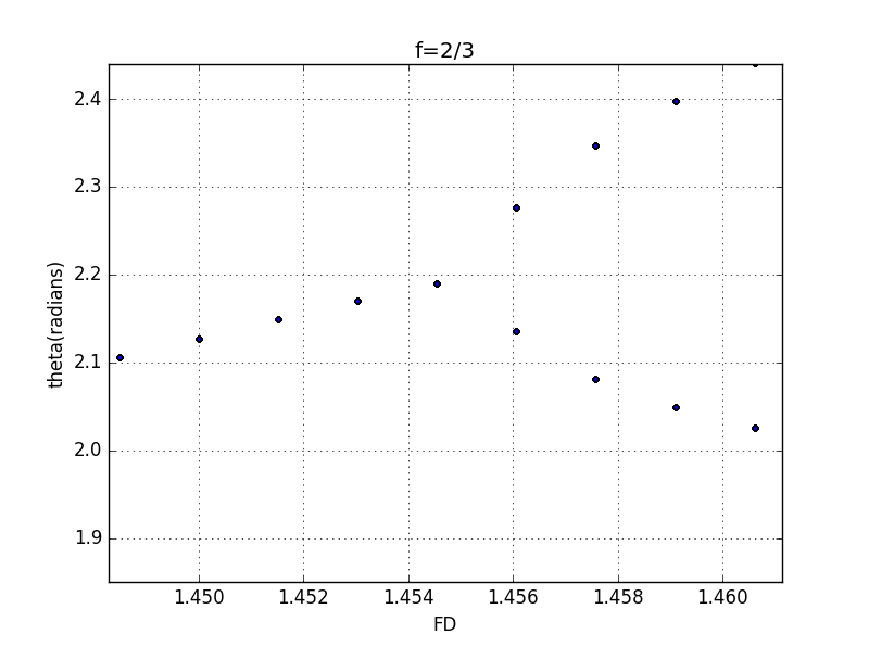
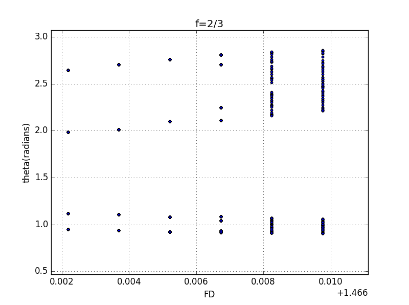
here,I can only distinguish three points,and their corresponding coordinates are 1.41972、1.45455、1.47123
$\delta_2=\frac{F_2-F_1}{F_3-F_2}$=2.088

Now ,I tend to Poincare sections for the pendulum as it undergoes the period-doubling route to chaos for$F_D=1.4　　F_D=1.44 　and　F_D=1.465$



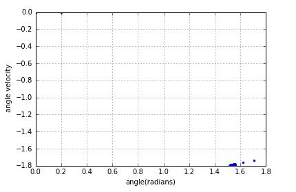
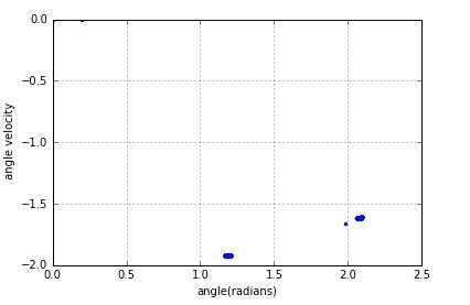
After removing the points corresponding to the initial transient the attractor in the period-1 regime will contain,likewise,the attractor will contain n discrete points if the behavior is period n.
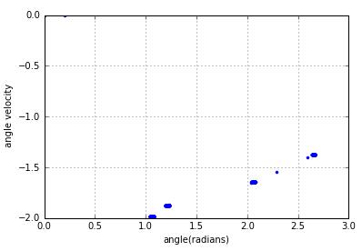
when change the driving force,I find a interesting phenomenon



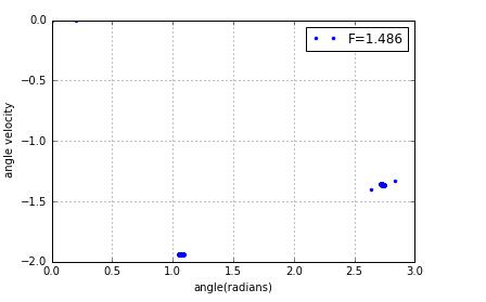
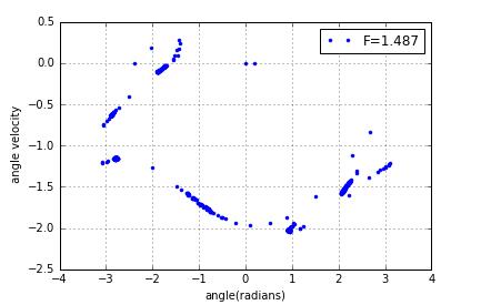
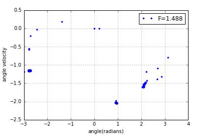
a small change to force will change the poincare sections a lot

In order to see this phenomenon clearly,we tend to observe bifurcation diagram by change the condition like the drive frequency and damping parameter.




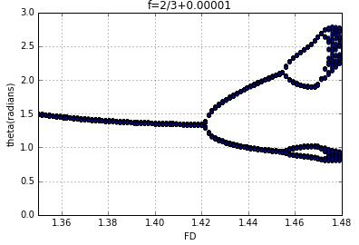
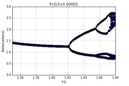
when the frequency increase a little,the figure move down

it is not a esay job, for the bifurcation diagram can easily be strange with a unsuitable frequency.

or change q,the parameter that measures the strength of the damping


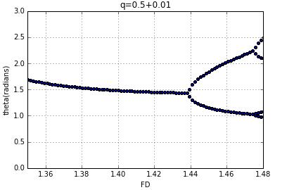
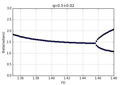
we can see that bifurcation point move right.
since drag force is larger,the drive force is increasing at the same time.

Conclusion

We have now obtained at least a qualitative understanding of how the transiton from rugular to chaotic behavior occurs for one particular systerm in one particular range of parameters.

Thanks

Douwei's support for vPython.
Wu yuqiao's code for vPython's show.