PRECESSION OF THE PERIHELION OF MERCURY

Precession is a common phenomenon in our life.
The object rotates while rotating around a fixed axis.This is a interesting experiment.At the same time astronomy is a precise science.We should know that most of the planets have orbits that are very nearly circular.The planets whose orbits deviate the most from circular are Mercury and Pluto.For Mercury the orientation of the axes of the ellipse that describes its orbit rotate with time.Different planets have differnt magnitude of this precession.For Mercury,the magnitude of this precession is approximately 566×1/3600 of a degree per century.

Until 1917,Einstein developed the theory of general relativity.
The force law predicted by general relativity is
$F_G=\frac{GM_SM_M}{R^2}(1+\frac{\alpha}{r^2})$
The approach we take here is to calculate the rate of precession as a function of $\alpha$

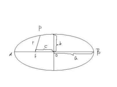
The length of the semimajor axis for Mercury's orbit is a=0.39AU

Conservation of total energy implies that the energies at points 1 and 2 are the same.Thus
$-\frac{CM_SM_M}{r_1}+1/2M_Mv_1^2=-\frac{CM_SM_M}{r_2}+1/2M_Mv_2^2$
the angular momentum at point 1 is equal to that at point 2,which yields $r_1v_1=r_2v_2$
For aphelion of mercury, the velocity is 8.2AU/yr,and the distance to sun is $r_1=(1+e)a=0.47AU$ and the distance of the perihelion is $r_2=(1-e)a=0.309AU$

from pylab import *
import matplotlib as mpl
from math import sqrt, pi
from mpl_toolkits.mplot3d import axes3d, Axes3D
import numpy as np
import matplotlib.pyplot as plt
class Mecury():
    def __init__(self, initx=0.47, inity=0, initvx=0, initvy=8.2, dt=0.001, powerlaw=2., alpha=0.008, outputfile=''):
        self.dt=dt
        self.beta=powerlaw
        self.alpha=alpha
        self.filename=outputfile
        self.calculate(sqrt(initx*initx+inity*inity), initx, inity, initvx, initvy, 0.)
        self.dth=0.
    def stepOne(self, r, x, y, vx, vy, t):
        r=sqrt(x*x+y*y) 
        vx=vx-(4*pi*pi*x*self.dt)/r**(self.beta+1)/(1+self.alpha/r**(self.beta))
        vy=vy-(4*pi*pi*y*self.dt)/r**(self.beta+1)/(1+self.alpha/r**(self.beta))
        x=x+vx*self.dt
        y=y+vy*self.dt
        t=t+self.dt
        return r, x, y, vx, vy, t
    def calculate(self, r, x ,y ,vx, vy, t):
        self.data=[(r, x,y,vx,vy,t)]
        while t<100:
            r, x, y, vx, vy, t=self.stepOne(r, x ,y ,vx, vy, t)
            self.data.append((r, x,y,vx,vy,t))
        if self.filename!='':
            self.store()
    def store(self):
        pass
    def plotMecury(self, figType=1):
        x=[]; y=[]; z=[0.]; vx=[]; vy=[]; t=[]; r=[]; xp=[]; yp=[]; k=[]
        for i in range(5000):
            (r1, x1, y1, vx1, vy1, t1)=self.data[i]
            x.append(x1); y.append(y1); vx.append(vx1); vy.append(vy1)
            t.append(t1); z.append(0.); r.append(r1)
            if i>2:
                dr1=r[i-1]-r[i-2]
                dr2=r[i]-r[i-1]
                if dr1>0 and dr2<0:
                    xp.append(x[i-1])
                    yp.append(y[i-1])
            m=len(self.data)
        if figType==1:
            plot(x,y)
            plot(0,0,'r*')
            for j in range(len(xp)):
                plot([0,xp[j]], [0,yp[j]],'k-')
            xlim(-0.55,0.55)
            ylim(-0.55,0.55)
            show()
        else:
            fig=plt.figure()
            ax=Axes3D(fig)
            ax.plot(x[0:m], y[0:m], z[0:m], label='Kepler')
            ax.legend()
            plt.show()
    def plotPrecessionrate(self, figType=1):
        x=[]; y=[]; z=[0.]; vx=[]; vy=[]; t=[]; r=[]; xp=[]; yp=[]; tp=[]; k=[];
        theta=[]; th=0.; dth=0.#dth=[]
        for i in range(3000):
            (r1, x1, y1, vx1, vy1, t1)=self.data[i]
            x.append(x1); y.append(y1); vx.append(vx1); vy.append(vy1)
            t.append(t1); z.append(0.); r.append(r1)
            if i>2:
                dr1=r[i-1]-r[i-2]
                dr2=r[i]-r[i-1]
                if dr1>0 and dr2<0:
                    xp.append(x[i-1])
                    yp.append(y[i-1])
                    tp.append(t[i-1]-0.24500000000000019)
            m=len(self.data)
            n=len(xp)
        if figType==1:
            for j in range(n):
                k.append(yp[j]/xp[j])
                theta.append((180/pi)*(arctan((k[0]-k[j])/(1+k[0]*k[j]))))
            for l in range(n-1):
                th=th+theta[l+1]/tp[l+1]
            dth=th/n
            print (theta)
            print (tp)
            print (dth)
            #print th
            #print theta[0]/tp[0]
            plot(tp,theta)
            #plot(0,0,'r*')
            xlim(0,3)
            ylim(0,20)
            show()
        else:
            fig=plt.figure()
            ax=Axes3D(fig)
            ax.plot(x[0:m], y[0:m], z[0:m], label='Kepler')
            ax.legend()
            plt.show()
        #return dth
    def calculatedth(self, figType=1):
        x=[]; y=[]; z=[0.]; vx=[]; vy=[]; t=[]; r=[]; xp=[]; yp=[]; tp=[]; k=[];
        theta=[]; th=0.; dth=0.#dth=[]
        for i in range(3000):
            (r1, x1, y1, vx1, vy1, t1)=self.data[i]
            x.append(x1); y.append(y1); vx.append(vx1); vy.append(vy1)
            t.append(t1); z.append(0.); r.append(r1)
            if i>2:
                dr1=r[i-1]-r[i-2]
                dr2=r[i]-r[i-1]
                if dr1>0 and dr2<0:
                    xp.append(x[i-1])
                    yp.append(y[i-1])
                    tp.append(t[i-1]-0.24500000000000019)
            m=len(self.data)
            n=len(xp)
        if figType==1:
            for j in range(n):
                k.append(yp[j]/xp[j])
                theta.append((180/pi)*(arctan((k[0]-k[j])/(1+k[0]*k[j]))))
            for l in range(n-1):
                th=th+theta[l+1]/tp[l+1]
            self.dth=th/n
def calculaterate():
    listalpha=[]
    listdth=[]
    list1=[0,1,2,4,8,16]
    rate=0.
    for k in range(6):
        list1[k]=0.0002*list1[k]
        c=Mecury(alpha=list1[k])
        c.calculatedth()
        listalpha.append(c.alpha)
        #print c.alpha
        listdth.append(c.dth)
        #print c.dth
    print (listalpha,listdth)    
    plot(listalpha, listdth, 'ro')
    for m in range(5):
        rate+=listdth[m+1]/listalpha[m+1]
    drate=rate/6
    print (drate)
    show()
a=Mecury(alpha=0.01)
a.plotMecury()
#b=Mecury(alpha=0.0008)
#b.plotPrecessionrate()
#calculaterate()

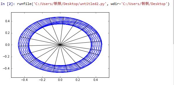
Clearly, this result is a little strange compared with other procession figure.

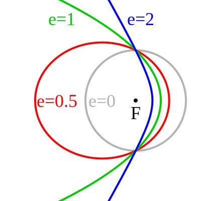
For a constant $\beta$ like 2.05 and a constant aphelion,change the eccentricity e.

code1.py

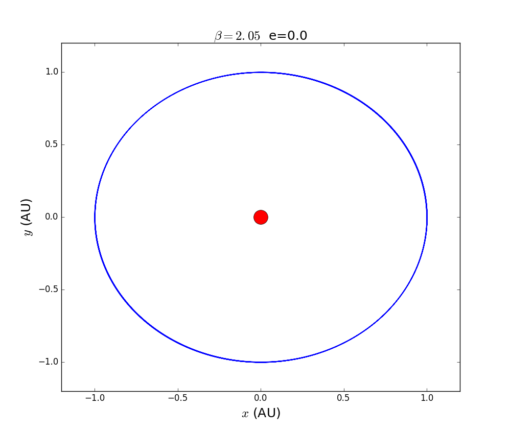
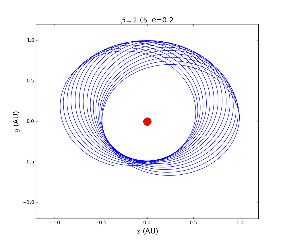
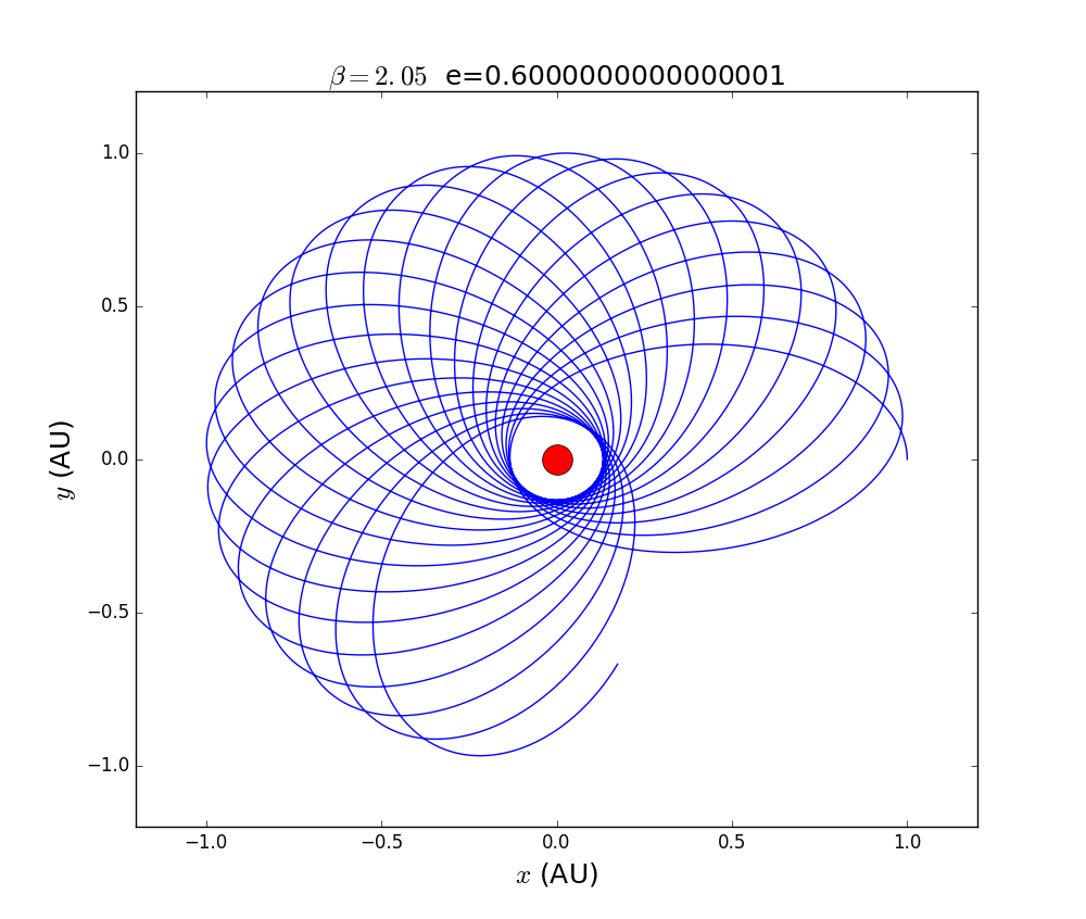
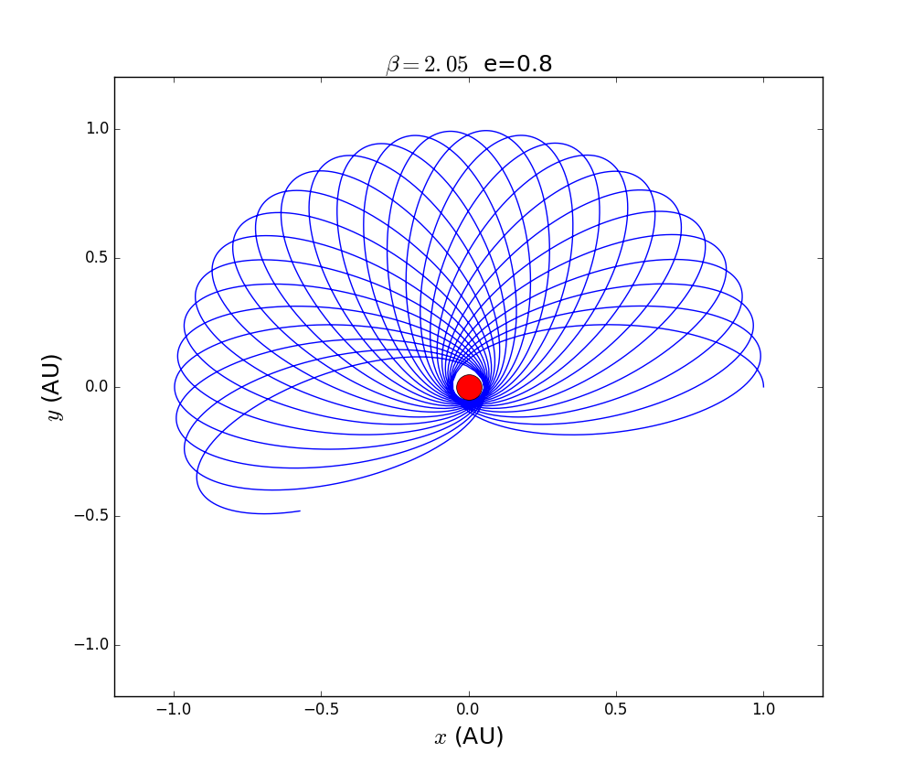
we include those figure into one gif.

we use the following figure to show the regularity.

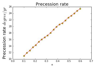
we can see the precession rate is increasing along the eccentricity.
of couse this is for orbit of ellipse but not for hyperbola and parabola

Conclusion

The homework talk about the orbit of solar systerm.By supposing that the law deviates slightly from an inverse_square dependence to discuss a possible way to occur precession.

Reference

Wikipedia
computational physics；Nicholas J. Giordano, Hisao Nakanishi.