View this on Github
View this on "作业部落"

Exercise 10: Lorenz Model

王世兴
2013301020050

---

Level 1

Construct the phase-space plots of Lorenz model in the different regimes.

---

Level 3

Display the results with VPython.

Background

Lorenz Model

The Lorenz system is a system of ordinary differential equations (the Lorenz equations, note it is not Lorentz) first studied by Edward Lorenz. It is notable for having chaotic solutions for certain parameter values and initial conditions. In particular, the Lorenz attractor is a set of chaotic solutions of the Lorenz system which, when plotted, resemble a butterfly or figure eight. [1]

Second-Order Runge-Kutta Method [2]

Although Euler and Euler-Crome method resemble the Taylor expansion of a function, at the first order, variance exists. But by the "mean value theorem", we can always find a point $t_m$ between $t$ and $t+dt$ such that

$$x(d+\Delta t)=x(t)+\frac{dx(t_m)}{dt}\Delta t$$
A more effective approxiamtion than Euler method can be constructed by estimating $t_m$ and $dx/dt|_{t_m}$. And the second-order Runge-Kutta method is such a way given by
$$x(t+\Delta t)=x(t)+f'(x',t')\Delta t$$
where
$$\begin{array}{rl}x'&=x(t)+\frac{1}{2}f(x(t),t)\Delta t\\t'&=t+\frac{1}{2}\Delta t\end{array}$$

Discussion: Main Features of the Program

Our program has the following advantages.

• Object-Oriented Manner
  We defined a class Lorenz to include the initialization of parameters, calculation of the differential equations, display of phase plots and 3D animation. This is extra conventient when we change the parameters and repeat the same processes.

• Seond-Order Runge-Kutta Method
  This time we use the second-order Runge-Kutta method to improve the accuracy of the results. The accuracy and stability of Rubge-Kutta mathods have been discussed throughly by my classmates. [3][4] We choose the second order as a balance between acccuracy and time-efficiency.

• Only One Cycle
  To obtain the attractor in chaos phemonenon, we need to get two of the coordinates when the third is zero. This means judging and cycle structure is inevitable in the program, which is a terrible time consumer. We solve this problem by combining choosing points for the attractor plot with solving differential equations. In this way can we use only one cycle to give all the plots needed, while the drawback is also obvious that this program may take more memory.

• Well-Selected Parameters
  At first the attractor plot is always not the same as that in the textbook. [2] The plot are separate into several discrete lines and the number of points are too little. It is due to the algorithm we use to judge x=0. As float numbers we can only assign a small intervel near zero to approximate x as zero. If the interval is too large, more points than wanted will to included as a short line. As we shrten the interval, more time steps are needed to gether enough points. The details of the selection of parameters are given under each plot we show in the next section.

Result

Firstly we repeat the process in the textbook [2] to confirm that our program is correct. The three-dimension phase plot is given below (Figure 10.1) and its projection onto three orthogonal plains are the same as Figure 3.16 in the textbook. [2]

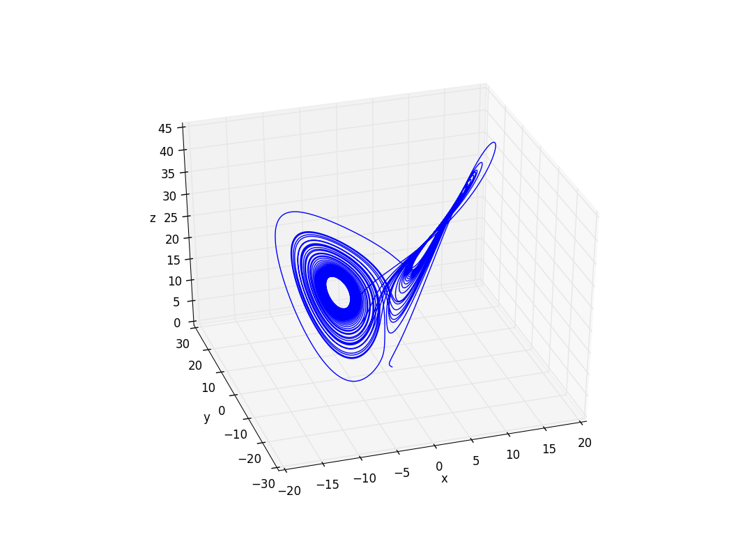
Figure 10.1 Three-diemensional phase plot with r=25, $\sigma=10$, b=8/3, dt=0.0001s, time=50s

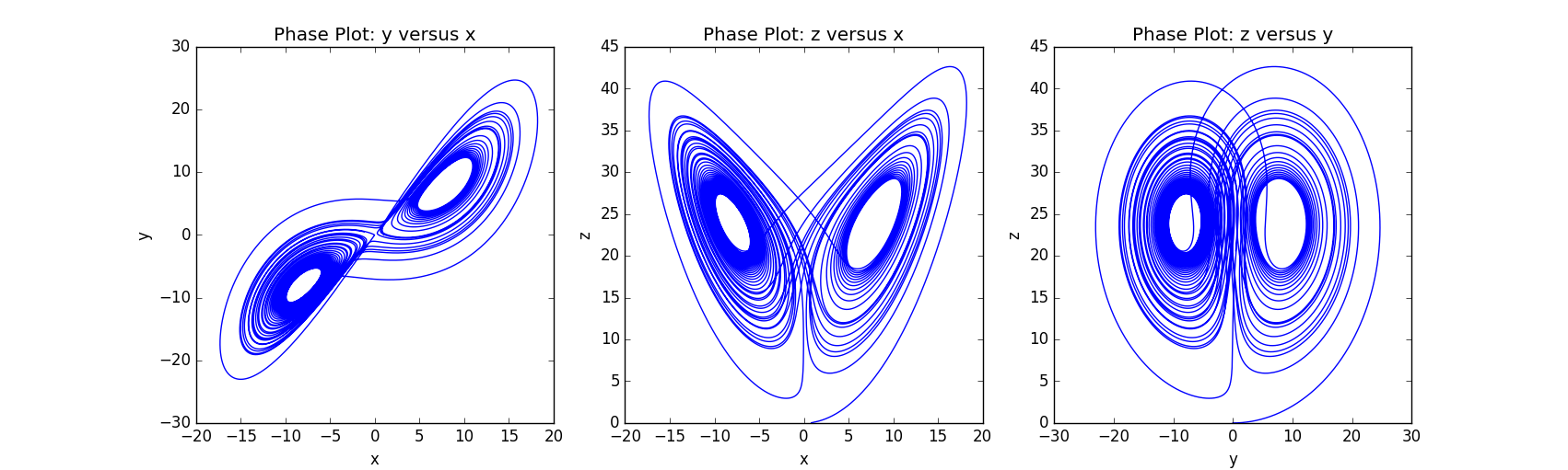
Figure 10.2 Phase plot projected onto xOy, xOz, yOz plain, with r=25, $\sigma=10$, b=8/3, dt=0.0001s, time=50s

To obtain the attractor we give up the points before t=30s and judge whether the x coordiante is within a small range near zero (-0.001,0.001). To get enough points we take a long time=1000s.

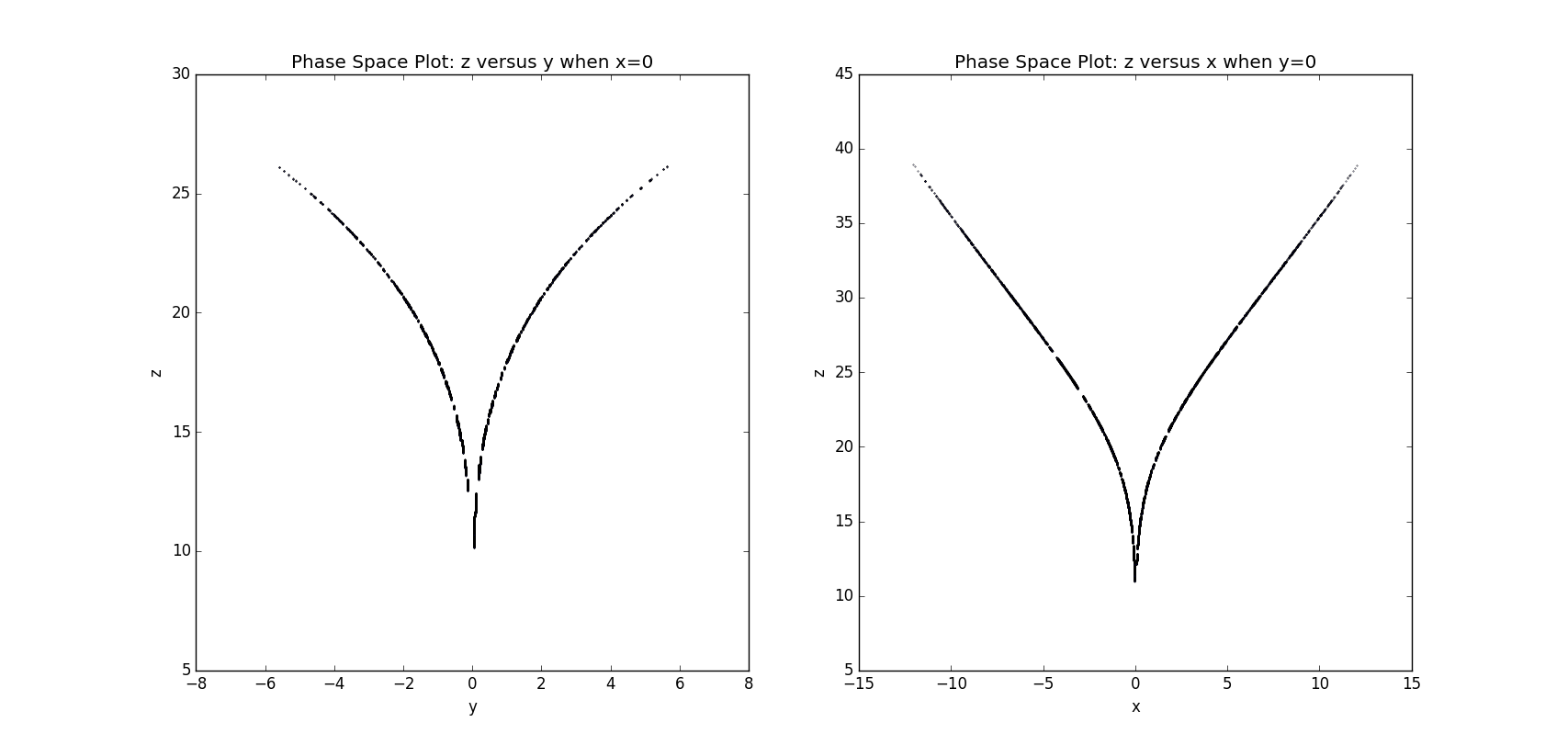
Figure 10.3 Attractors when x=0 (left) and y=0 (right), with r=25, $\sigma=10$, b=8/3, dt=0.0001s, time=50s

Thus we are confident to claim that we get the correct code to go further. According to the requirement of question 3.26 we choose several different r to give the phase plot onto xOz plain and the attractors.

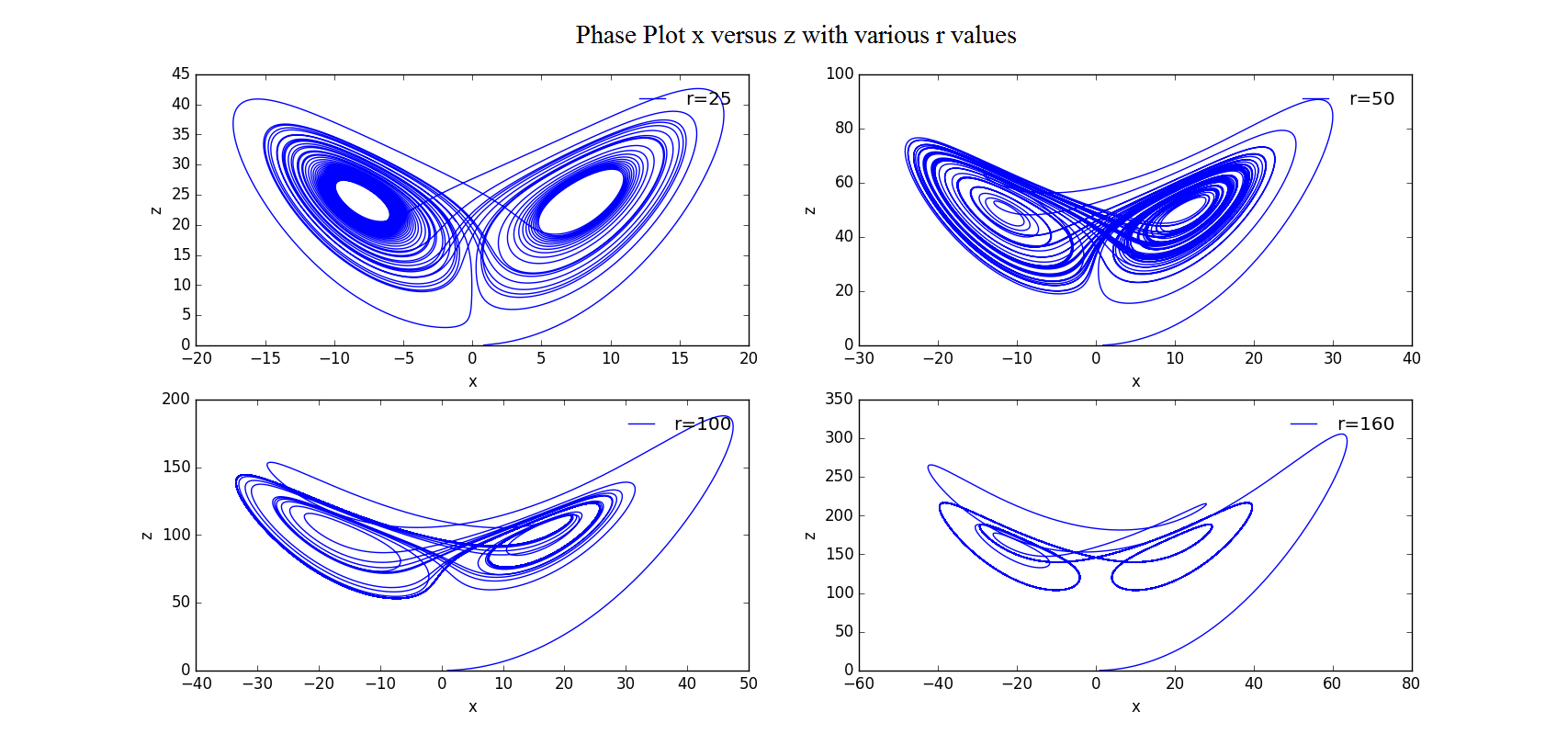
Figure 10.4 Phase plot projected onto xOz plain, with r=25, $\sigma=10$, b=8/3, dt=0.0001s, time=50s

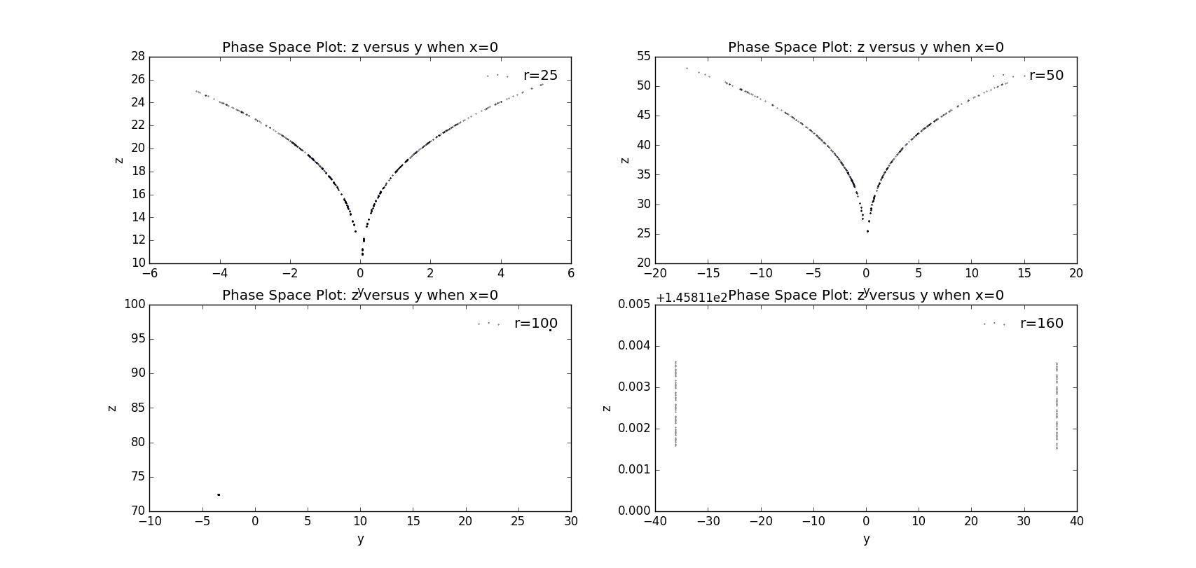
Figure 10.5 Attractors when x=0 with various r values, with r=25, $\sigma=10$, b=8/3, dt=0.0001s, time=50s

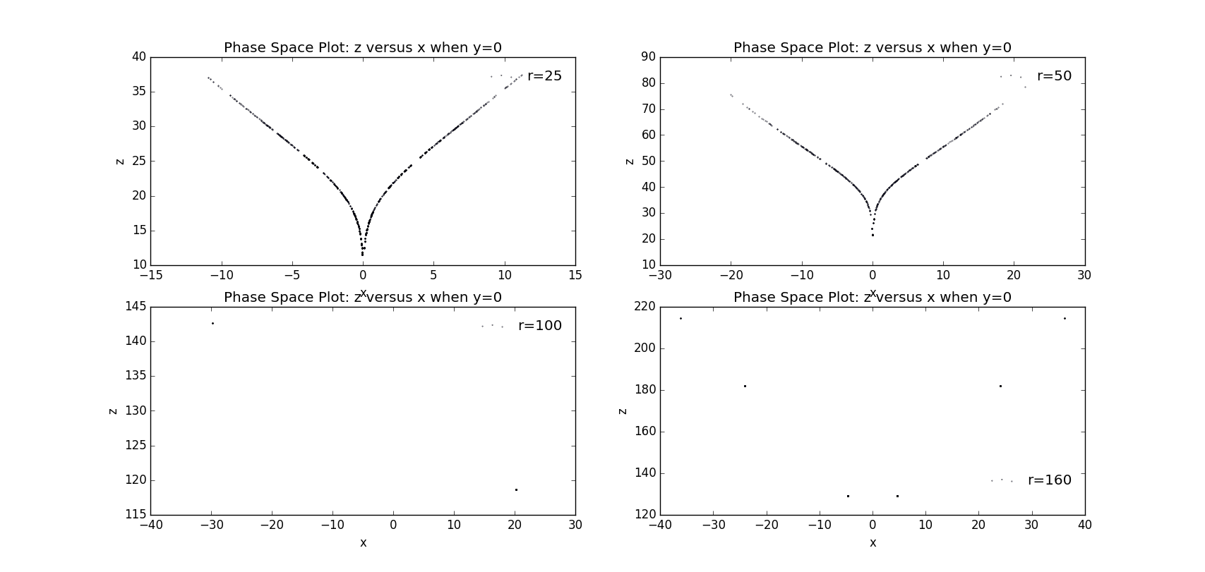
Figure 10.6 Attractors when y=0 with various r values, with r=25, $\sigma=10$, b=8/3, dt=0.0001s, time=50s

Reference

1. Wikipedia contributors. "Lorenz system." Wikipedia, The Free Encyclopedia. Wikipedia, The Free Encyclopedia, 24 Apr. 2016. Web. 2 May. 2016.

2. Giodano, N.J., Nakanishi, H. Computational Physics. Tsinghua University Press, December 2007

3. 陈洋遥. "计算物理第8次作业　振动：Oscillatory Motion". https://www.zybuluo.com/cyy652415049/note/347388, 2016-04-19

4. 陈锋. "Instruction of ode.py". https://www.zybuluo.com/355073677/note/323818, 2016-03-26