First written with Jupyter.
The differential equation codes can be found here and the subplot codes here.

Exercise 4 - Double Decay

Abstract

Although it has been the ultimate goal for scientists to find the analytical solution of the nature, some complicated sysyems still hinder people from this dream in which circumstances numerical methods are necessary. Ordinary differential equations are good practice for us to get familiar with the numerical methods, for we can compare our result with the known analytical solution. In this problem, we consider a system in which The errors for ingoring high rank differentiation may sometimes make such methods invalid, so various initial conditions and parameters are discussed to examine the sensitivity of the parameters and the rubustness of the method.

Background

Ordinary Differential Equation [1]

The categories of equations are based on the type of known quantities and the calculation on the unknown quantities. The equations are called algebraic equtions or transcedent equations if the unknown quantities are numbers. An equation is called a function equation if the unknown quantity is a function. It is called a differential equation if there are derivative or differential in an equation, among which the ones containing functions with only one variables are called the ordinary differential equations.

And as is proven, the theorem about the existence and uniqueness of the solution says for a differential equation $\frac{dy}{dx}=f(x,y)$
with the boundary condition $y(x_0)=y_0$, the solution exists and is unique if in the region

$$R:x_0 -a \leq x \leq x_0 + a,\ y_0 -b \leq y \leq y_0+b$$
(1) f(x,y) is continuous.
(2) f(x,y) satisfies the Lipschitz condition about y, which means for any pair of points $(x,y)$ and $(x,\bar y)$, there exists N such that
$$|f(x,y)-f(x, \bar y)| \leq N |y-\bar y|$$
This theorem provides us with confidence about the solution we find. Once it satisfys the differential conditions of thq equation, it much be the correct and the only correct solution.

Euler Methods

As we know, any real or complex function that can be differentiated to infinite orders at point $x_0$ can be represented as an infinite sum of about the differentials like

$$f(x)=\sum_{n=0}^\infty \frac{f^{(n)}(x_0)}{n!}(x-x_0)^n=x_0+f'(x_0)(x-x_0)+\frac{1}{2}f''(x_0)(x-x_0)^2+...$$
This theorem has provided us with a way to approximate a function in forms of a poynomial function, which can be easily calculated in computers. [2][3]Especially, if we ignore the differentials greater than the second order, which means
$$f(x) \approx f(x_0)+\frac{df(x_0)}{dx}(x-x_0)$$
This method to figure out the approximate solution is called the Euler method.
Suppose the function $f(x,y)$ is continuous and bounded in the region $a \leq b, |y| <\infty$,then $f(x,y)$ determines a direction field. To get the approximate solution of the ordinary equation with boundary condition
$$\begin{array}{ll} \frac{dy}{dx}=f(x,y) \\ y(x_0)=y_0 \end{array}$$
divide the interval $[x_0,b]$ into n equal pieces,and the dividing points are
$$x_k=x_0+kh,\ \ k=0,1,...,n$$
$$h-\frac{b-x_0}{n},\ \ x_n=b$$
Because the tangent of the solution at the point $(x_0,y_0)$ should be f(x_0,y_0), we use the straight line passing (x_0,y_0) with the tangent f(x_0,y_0) as an approximaiton of the curve. The function of the straight line is
$$y=y_0+f(x_0,y_0)(x-x_0)$$
And the y-coordinate $y_1$ of the straight line at the point $x_0$ should be
$$y_1=y_0+f(x_0,y_0)(x_1-x_0)=y_0+f(x_0,y_0)h$$
If $h$ is very small, then $y_1 \approx y(x_1)$, thus the point $(x_1,y_1)$ is fairly close to the point on the solution curve. If $f(x,y)$ is continuous, then the straight line starting from $(x_1,y_1)$ approximates the solution curve， with the function
$$y=y_1+f(x_1,y_1)(x-x_1)$$
And the y-coordinate of the end of this straight line is
$$y_2=y_1+f(x_1,y_1)(x_2-x_1)$$
And the rest can be done in the same manner,
$$y_k=y_{k-1}+f(x_{k-1},y_{n-1})(x_{k}-x_{k-1})$$
Since the function of every straight line is known, so for every point in the interval $[x_0,b]$, we can figure out the approxiamtion of the solution $y=y(x)$. And the fold line as the approximation of the solution is called the Euler Fold Line. It can be proven that when $n$ approaches infinity and $h$ approaches zero, the Euler fold line approaches the solution. [1]

Sensitivity and Robustness of Parameters [4]

What we have and will be doing in this exercise has little to do with first principles of physics. Rather, they are just methematical modelling problems. As a result, it is necessary to discuss the sensitivity and robustness, two of the essential concepts in mathematical modelling.

To set up a model describing a phenomenon, parameters play an important role in the final results of the model. These parameters are obtained from measurements, observations, and sometimes even by guess. So the inaccuracy of the data must be taken into consideration. Usually, for a certain extent of change of a parameter, the variable will change correspondingly. For the parameter $r$ and the variable $x$,

$$\lim_{\Delta r \rightarrow 0}\frac{\Delta x / x}{\Delta r / r}=\frac{dx}{dr} \frac{r}{x}$$
And we call this limit the sensitivity of $x$ about $r$

A mathematical model is called robust if the result is still correct even if the model is not absolutely accurate. Sensitivity is a kind of index to evaluate the robustness of the model based on the data. Other assumptions will also be examined to ensure the robustness.

In most questions after Chapter 1 of our textbook, we have been informed of the models to use and only have to realize the model through Python and cast the parameters into the program. So the sensitivity and robustness of our parameters become important.

Imaging with Python

It is convenient to draw plots with Python, since there have been the powerful packages numpy and matplotlib.

numpy is a package that can deal with the discrete calculations that will be used in the ploting. Not only can it create number lists with the function arrange and linspace, it also contains the general math functions like the triangluar function sin cos.[5]

matplotlib is the package that deal with the representation of plots. [6] Through the internal functions we can easily And other information about this package and the rebellish of pots can be found here.

Program

Problem 1.5

Consider again a decay problem with two types of nuclei A and B, but now suppose that nuclei of typw A decay into type B, while nuclei of type B decay into type A. Strictly speaking, this is not a "decay" process, since it is possible for the type B nuclei to turn back into type A. A better analogy would be a resonance in which a system can tunnel or move back and forth between two states A and B which have equal energies. The corresponding rate equations are

$$\frac{dN_A}{dt}=\frac{N_B}{\tau}-\frac{N_A}{\tau}$$
$$\frac{dN_B}{dt}=\frac{N_A}{\tau}-\frac{N_B}{\tau}$$
where for simplicity we have assumed that the two types of decay are characterized by the same time constant $\tau$. Solve the system of equations for the numbers of nuclei, $N_A,N_B$ as functions of time. Consider different initial confitions, such as $N_A=100,\ N_B=0$ etc, and take $\tau=1s$. Show that your numerical results are consistent with the idea that the system reaches a steady state in which $N_A,N_B$ are constant. In such a steady state, the time derivatives $dN_A / dt,\ dN_B / dt$ should vanish.

Declear and Initialize Variables and Parameters

Apparently the decay constants of A and B are important parameters. Here we have assumed that the two parameters equal. However, they do not necessarily have to be, so we declear $\tau_A$ and $\tau_B$ as separate parameters and initialize them with the same quantity.
Another parameter is the time interval for the Euler fold line to approximate the "true" solution of the equations. Apparently the smaller this parameter dt is, the closer our numerical solution will approach the true solution, but the slower the program will be. For convenience we set $dt\ =\ 0.1\ second$ and will examine the effect of it value in the Discussion section.
And as an intuition, the system will become stable after certain amount of time. So we need a parameter timescale to control the time we want the system to develop.

As for the variables, the solutions are the function $N_A(t)$ and $N_B(t)$. So we need two lists to store the value of $N_A$ and $N_B$ and a time list which has the same length of $N_A$ and $N_B$. The initial conditions are initialized as the first element of the lists.

Calculation

The algorithm of the problem is straightforward. We set up a cycle in which the new $N_A$ and $N_B$ value is obtained from the value of $N_A$ and $N_B$ before the time interval plus the product of the time interval and the derivative of $N_A$ and $N_B$ versus time.

Represent and Restore the Results

Since the function $N_A$ and $N_B$ has been stored into the lists, we can plot them with the help of package matplotlib

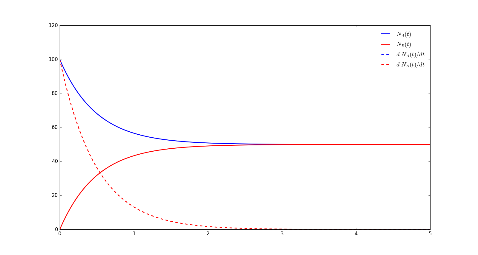
The $dN_A(t)$ curve cannot be seen because it is below the x-axis. And it should be the mirror refelction of $dN_B(t)$(the proof is shown below).

Discussion

Comparasion with Analytical Solution

According to the eigenvector mathod we can solve such ordinary differential equations fairly easily. For the equations with the boundary conditions

$$\begin{array}{llll}\frac{dN_A}{dt}=\frac{N_B}{\tau_2}-\frac{N_A}{\tau_1}\\ \frac{dN_B}{dt}=\frac{N_A}{\tau_1}-\frac{N_B}{\tau_2}\\ N_A(0)=N_{A_0}\\ N_B(0)=N_{B_0}\end{array}$$
The analytical solution would be
$$\begin{array}{ll}N_A(t)= \frac{(N_{A_0}+N_{B_0})\tau_1}{\tau_1+\tau_2}+\frac{-N_{B_0}\tau_1+N_{A_0}\tau_2}{\tau_1+\tau_2}e^{-(\frac{1}{\tau_1}+\frac{1}{\tau_2})t}\\ N_B(t)= \frac{(N_{A_0}+N_{B_0})\tau_2}{\tau_1+\tau_2}+\frac{N_{B_0}\tau_1-N_{A_0}\tau_2}{\tau_1+\tau_2}e^{-(\frac{1}{\tau_1}+\frac{1}{\tau_2})t}\end{array}$$

Our numerical solution show a exponential feature and the derivative about time vanish as time approaches infinity. And the

This means the tendency of $N_A(t)$ and $N_B(t)$ depends on which of the two quantities $N_{B_0}\tau_1$ and $N_{A_0}\tau_2$ is greater. If the former is greater, then $N_A(t)$ decreases and $N_B(t)$ increases, and vice versa. And remind that at every time $N_A+N_B=const.$ So this process can also be treated as an exchange of states for a certain matter.

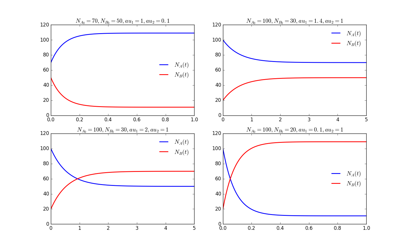
To draw several figures in the same picture we need the function subplot, and the settings of the ticks and limits of x-axis and y-axis are slightly different with plot function.

Sensitivity Analysis: How Will the Curve Shifts as Parameters Change?

Sensitivity of the Final Number about the Decay Constant

According to the analytical solution, the number of A and B at the final state

$$N_A(\infty)=\lim_{t \to \infty}N_A(t)=(N_{A_0}+N_{B_0})\frac{\tau_1}{\tau_1+\tau_2}$$
$$N_B(\infty)=\lim_{t\to\infty}N_B(t)=(N_{A_0}+N_{B_0})\frac{\tau_2}{\tau_1+\tau_2}$$
The effect of the initial number of both matter is obviously linear, and the sensitivity will increase a little bit as $N_A$ and $N_B$ increase. This is because the respond of the final number is always smaller than the change of initial state.

Here we choose the same decay constant ($\tau_1=\tau_2=1s$) and fix $N_B(0)=0$, to get the effect of different $N_{A_0}$

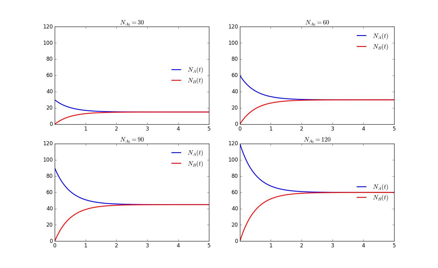
According to the Reference [4], the sensitivity of A and B about $\tau_1$ and $\tau_2$

$$Sen(N_A(\infty),\tau_1)=\frac{\partial N_A(\infty)}{\partial \tau_1}\frac{\tau_1}{N_A(\infty)}=\frac{\tau_2}{\tau_1+\tau_2}$$
$$Sen(N_A(\infty),\tau_2)=\frac{\partial N_A(\infty)}{\partial \tau_2}\frac{\tau_2}{N_A(\infty)}=-\frac{\tau_1}{\tau_1+\tau_2}$$
$$Sen(N_B(\infty),\tau_1)=\frac{\partial N_B(\infty)}{\partial \tau_1}\frac{\tau_1}{N_B(\infty)}=\frac{\tau_1}{\tau_1+\tau_2}$$
$$Sen(N_A(\infty),\tau_2)=\frac{\partial N_B(\infty)}{\partial \tau_2}\frac{\tau_2}{N_B(\infty)}=-\frac{\tau_2}{\tau_1+\tau_2}$$

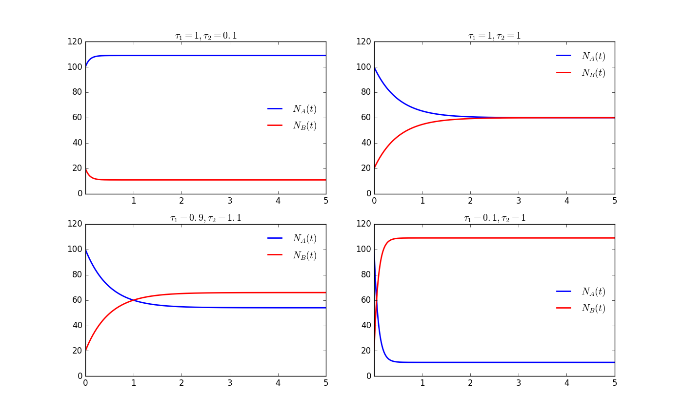
This means the sensitivities can never be over 1, and are independent with the initial number.

Here we fix $N_{A_0}=100,\ N_{B_0}=0$ and use various $\tau_1$ and $\tau_2$

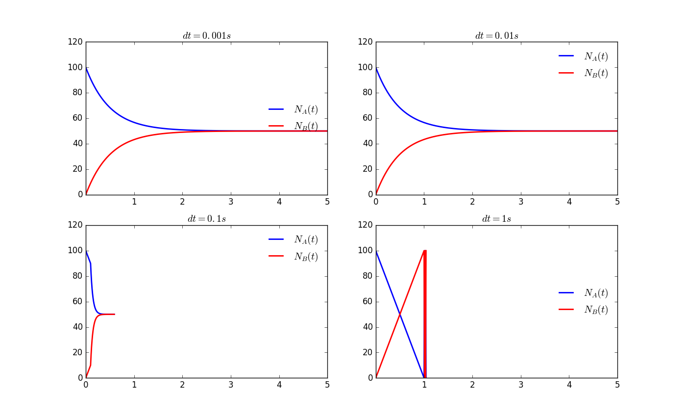
Robustness Analysis: Does Time Steplength Matter?

As is introduced in the Background section, the validity of Euler method depends on the Euler fold line as the approximation of the true solution curve. Specifically, it depends on the fact that the iterating interval is ralatively small comparing to the system of interest. But how big can this interval be? We tried several length of interval and the resluts are shown below.

Acknowledgement

All the codes and report are written by myself.
I must give my appreciation to FC Bayern Munchen club for their exciting victory in Allianz Arena against Juventus. They gave me an excellent weekend so that I can finish this exercise joyfully! Really looking forward to their highlight performance in Milan!

MIA SAN MIA!

Reference

[1] Differential Equation Group of Northeast University. Ordinary Differential Equation, Second Edition. Higher Education Press, April 2005.

[2] Qi, Minyou et al. Advanced Mathematics. Wuhan University Press, August 2008.

[3] Wikipedia contributors. "Taylor series." Wikipedia, The Free Encyclopedia. Wikipedia, The Free Encyclopedia, 20 Mar. 2016. Web. 22 Mar. 2016.

[4] Meerschaert, Mark M. Mathematical Modelling,Fourth Edition. China Machine Press, Janurary 1, 2015.

[5] "lectery", a Baidu user. Maypoltlib Guidebook.
http://wenku.baidu.com/link?url=haYK7EyFYYblwual6X1lAihWbvIFvYWx2MvEclbgARNn76kNJO9kU0Fb6R40YPuA71iHk60fD7HX_9PCaDTTuulVSRLcQwopIngL6uZjNpW

[6] Nicolas P. Rougier. Matplotlib Tutorial. http://www.labri.fr/perso/nrougier/teaching/matplotlib/