Chapter 7 Random System

1.Random Walk

A random walk is a mathematical object which describes a path that consists of a succession of random steps.

1.1 One-dimensional random walk

An elementary example of a random walk is the random walk on the integer number line , which starts at 0 and at each step moves +1 or −1 with equal probability.

• 

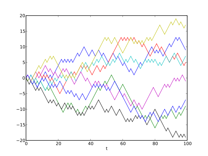
   Example of eight random walks in one dimension starting at 0. The plot shows the current position on the line (vertical axis) versus the time steps (horizontal axis).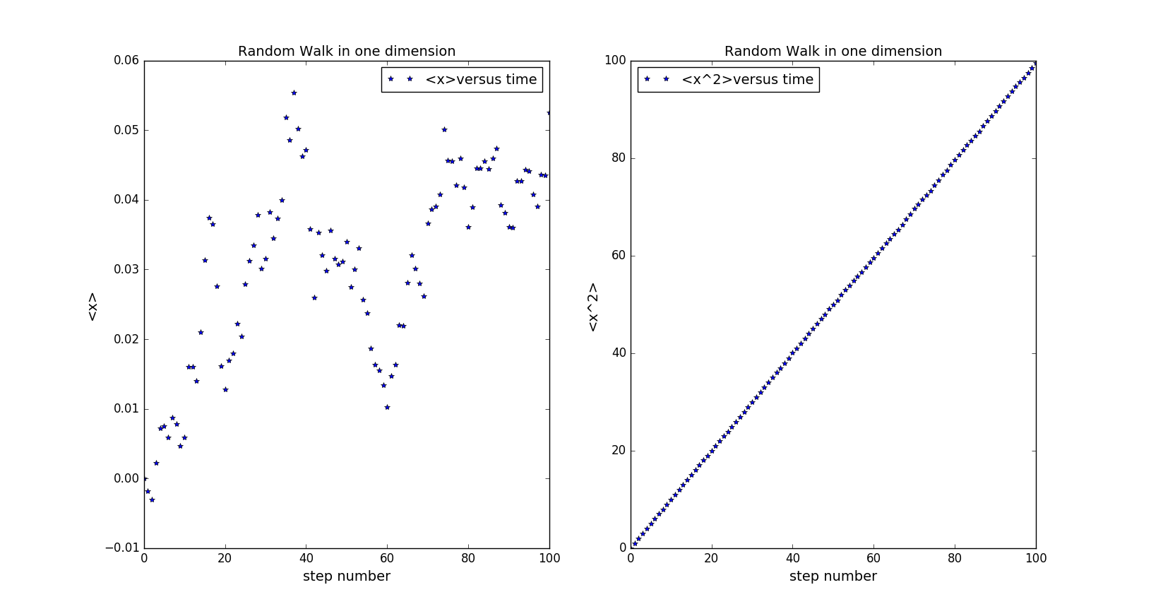
  

• 

This graph shows the average value of $x$ and $x^2$ after repeating the program for 50000 times. From the graph, we can conclude that approximates to 0 as we predicted and is linear to the step number(time). x=2Dt. In this graph, $D\approx0.5$ .

    Next change the step size from 1 to 0~1. See the change in D.

-

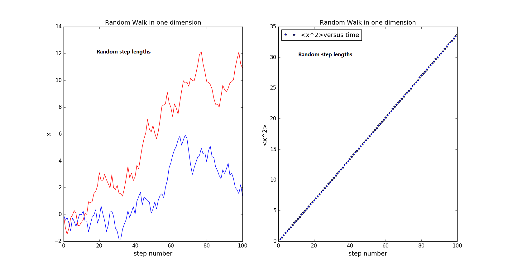
    As the step size becomes random, D decreases to approximately 0.175.

Code 1

Random walks in two dimension
three dimension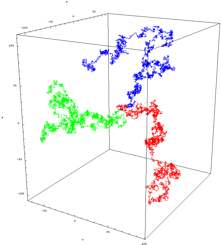

a display of particles' random walk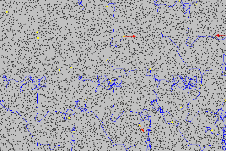

2.Self-avoiding Walks

In mathematics, a self-avoiding walk (SAW) is a sequence of moves on a lattice (a lattice path) that does not visit the same point more than once.

    Let's think about something more simplified--changing the probability of the each side.

• 

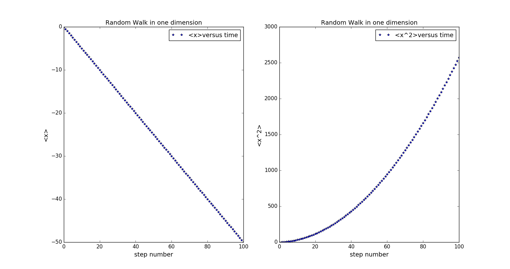
  The probability of stepping right is changed to 0.25.
  From the picture, we can see that <x> is linear to the time and <x^2> seems linear to the square of 
  

3.Random walks and Diffusion

Random walk are equivalent to diffusion.
In one dimension,$\frac{\partial \rho}{\partial t}=D\nabla ^2\rho$. According to the equation, $\rho(i,n+1)=\rho(i,n)+\frac{D\Delta t}{(\Delta x)^2}[\rho(i+1,n)+\rho(i-1,n)-2\rho(i,n)]$. Based on the equation above, we can use the programme to see the properties of $\rho$

    The graph below shows the changes of the density of the spots in one dimension when the time is varying.

• 

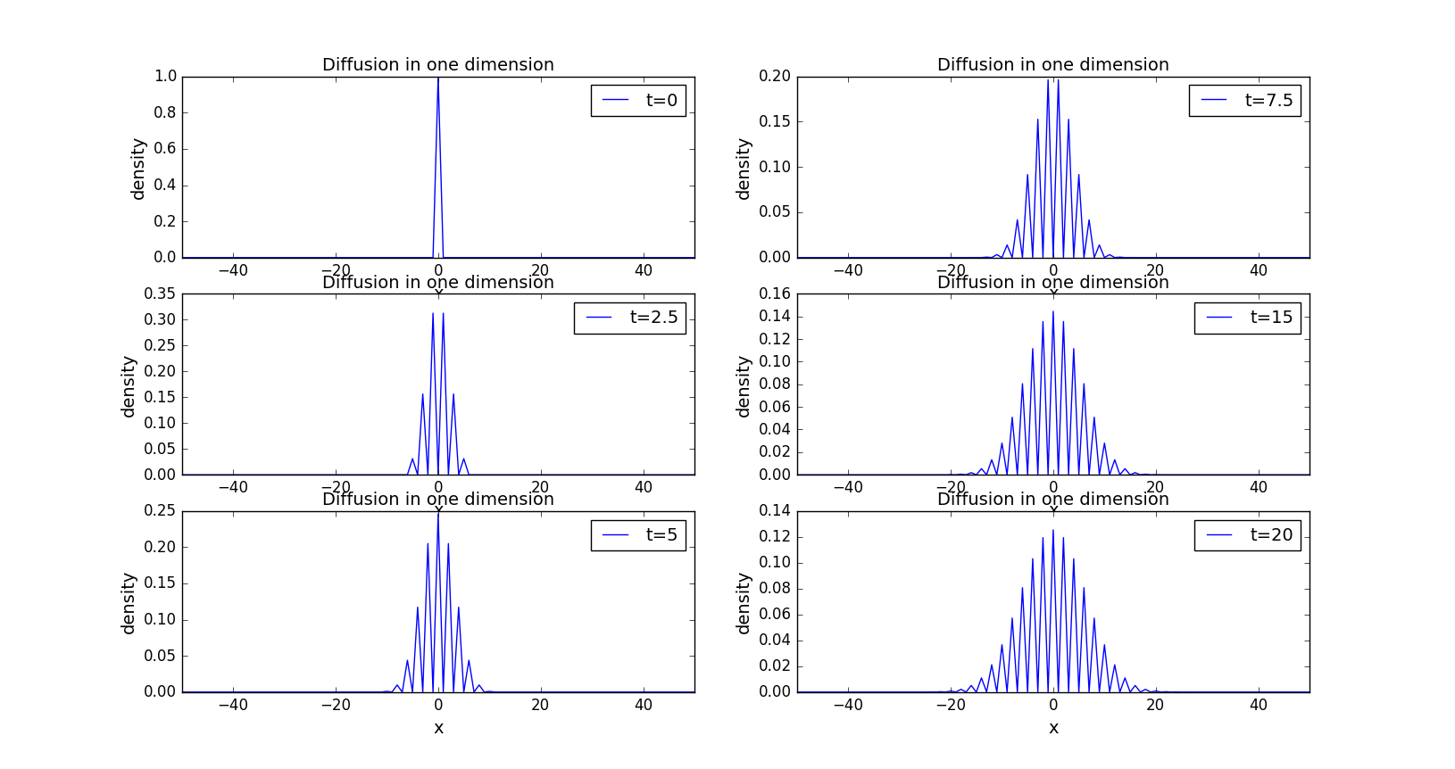
  As we can see, the curves satisfy the Gaussian distribution. 
  

Time evolution from the diffusion in two dimension

-

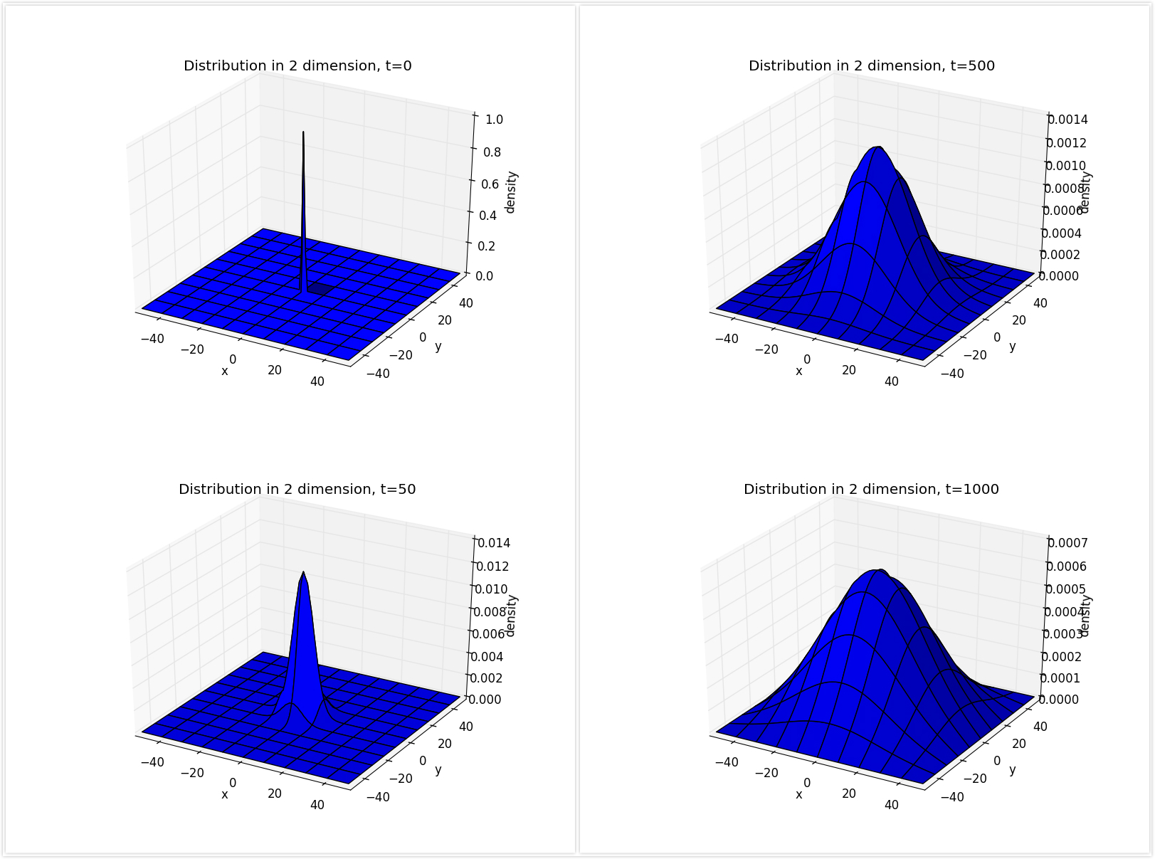
    The situation is similiar to that in one dimension.

code2

4.Cream-in-coffee

It is a two dimension random walk problem. First we set a number of particles in the center of the whole area. Then let them do random walks in all direction. The only limit is once they are reach the edge of the area they can not pass it. Then we observe how the particles move in different time.

-

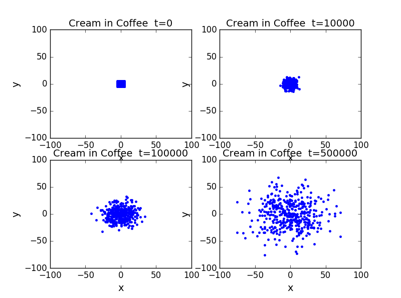
    As the steps increase, the particles gradually spread the whole area.

code3

In order to find the entropy of the system, we set the particles in different cells and then calculate $S=-\Sigma P_ilnP_i$.

-

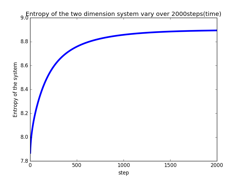
    As the steps increase, the entropy of the system increases nolinearly.

code4

Conclusion

    From the simulation of random walk, we can get the relationship between <x^2> and time.  We can also see the relationship between random walk and diffusion and how a diffusion process proceeds as time goes. From the last part, we can conclude that the entropy of a system always tends to increase as we learn from thermodynamics.