第十三课：法线贴图

OpenGL 教程

欢迎来到第十三课！今天的内容是法线贴图（normal mapping）。

学完第八课：基本着色后，我们知道了如何用三角形法线得到不错的着色效果。需要注意的是，截至目前，每个顶点仅有一条法线。在三角形内部，法线是平滑过渡的，而颜色则是通过纹理采样得到的（译注：三角形内部法线由插值计算得出，颜色则是直接从纹理取数据）。法线贴图的基本思想就是像纹理采样一样为法线取值。

法线纹理

下图是一张法线纹理：

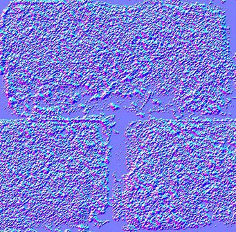
每个纹素的RGB值实际上表示的是XYZ向量：颜色的分量取值范围为0到1，而向量的分量取值范围是-1到1；可以建立从纹素到法线的简单映射：

normal = (2*color)-1 // on each component

由于法线基本都是指向“曲面外侧”的（按照惯例，X轴朝右，Y轴朝上），因此法线纹理整体呈蓝色。

法线纹理的映射方式和漫反射纹理相似。麻烦之处在于如何将法线从各三角形局部空间（切线空间tangent space，亦称图像空间image space）变换到模型空间（着色计算所采用的空间）。

切线和副切线（Tangent and Bitangent）

大家对矩阵已经十分熟悉了，应该知道定义一个空间（本例是切线空间）需要三个向量。现在Up向量已经有了，即法线：可用Blender生成，或由一个简单的叉乘计算得到。下图中蓝色箭头代表法线（法线贴图整体颜色也恰好是蓝色）。

然后是切线T：垂直于法线的向量。但这样的切线有很多个：

这么多切线中该选哪个呢？理论上哪一个都行。但我们必须保持连续一致性，以免衔接处出现瑕疵。标准的做法是将切线方向和纹理空间对齐：

定义一组基需要三个向量，因此我们还得计算副切线B（本可以随便选一条切线，但选定垂直于另外两条轴的切线，计算会方便些）。

算法如下：记三角形的两条边为deltaPos1和deltaPos2，deltaUV1和deltaUV2是对应的UV坐标下的差值；则问题可用如下方程表示：

deltaPos1 = deltaUV1.x * T + deltaUV1.y * B
deltaPos2 = deltaUV2.x * T + deltaUV2.y * B

求解T和B就得到了切线和副切线！（代码见下文）

已知T、B、N向量之后，即可得下面这个漂亮的矩阵，完成从切线空间到模型空间的变换：

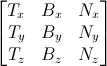
有了TBN矩阵，我们就能把（从法线纹理中获取的）法线变换到模型空间。

可我们需要的却是从切线空间到模型空间的变换，法线则保持不变。所有计算均在切线空间中进行，不会对其他计算产生影响。

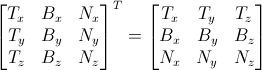
只需对上述矩阵求逆即可得逆变换。这个矩阵（正交阵，即各向量相互正交的矩阵，参见下文“延伸阅读”小节）的逆矩阵恰好也就是其转置矩阵，计算十分简单：

invTBN = transpose(TBN)

亦即：

准备VBO

计算切线和副切线

我们需要为整个模型计算切线、副切线和法线。我们用一个单独的函数完成这些计算：

void computeTangentBasis(
    // inputs
    std::vector<glm::vec3> & vertices,
    std::vector<glm::vec2> & uvs,
    std::vector<glm::vec3> & normals,
    // outputs
    std::vector<glm::vec3> & tangents,
    std::vector<glm::vec3> & bitangents
){

为每个三角形计算边（deltaPos）和deltaUV

    for ( int i=0; i<vertices.size(); i+=3){
        // Shortcuts for vertices
        glm::vec3 & v0 = vertices[i+0];
        glm::vec3 & v1 = vertices[i+1];
        glm::vec3 & v2 = vertices[i+2];
        // Shortcuts for UVs
        glm::vec2 & uv0 = uvs[i+0];
        glm::vec2 & uv1 = uvs[i+1];
        glm::vec2 & uv2 = uvs[i+2];
        // Edges of the triangle : postion delta
        glm::vec3 deltaPos1 = v1-v0;
        glm::vec3 deltaPos2 = v2-v0;
        // UV delta
        glm::vec2 deltaUV1 = uv1-uv0;
        glm::vec2 deltaUV2 = uv2-uv0;

现在用公式来算切线和副切线：

        float r = 1.0f / (deltaUV1.x * deltaUV2.y - deltaUV1.y * deltaUV2.x);
        glm::vec3 tangent = (deltaPos1 * deltaUV2.y   - deltaPos2 * deltaUV1.y)*r;
        glm::vec3 bitangent = (deltaPos2 * deltaUV1.x   - deltaPos1 * deltaUV2.x)*r;

最后，把这些切线和副切线缓存起来。记住，我们还没为这些缓存的数据生成索引，因此每个顶点都有一份拷贝。

        // Set the same tangent for all three vertices of the triangle.
        // They will be merged later, in vboindexer.cpp
        tangents.push_back(tangent);
        tangents.push_back(tangent);
        tangents.push_back(tangent);
        // Same thing for binormals
        bitangents.push_back(bitangent);
        bitangents.push_back(bitangent);
        bitangents.push_back(bitangent);
    }

索引

索引VBO的方法和之前类似，仅有些许不同。

找到相似顶点（相同的坐标、法线、纹理坐标）后，我们不直接用它的切线、副法线，而是取其均值。因此，只需把老代码修改一下：

        // Try to find a similar vertex in out_XXXX
        unsigned int index;
        bool found = getSimilarVertexIndex(in_vertices[i], in_uvs[i], in_normals[i],     out_vertices, out_uvs, out_normals, index);
        if ( found ){ // A similar vertex is already in the VBO, use it instead !
            out_indices.push_back( index );
            // Average the tangents and the bitangents
            out_tangents[index] += in_tangents[i];
            out_bitangents[index] += in_bitangents[i];
        }else{ // If not, it needs to be added in the output data.
            // Do as usual
            [...]
        }

注意，这里没有对结果归一化。这种做法十分便利。由于小三角形的切线、副切线向量较小；相对于大三角形来说，对模型外观的影响程度较小。

着色器

新增缓冲和uniform变量

我们需要再加两个缓冲，分别存储切线和副切线：

    GLuint tangentbuffer;
    glGenBuffers(1, &tangentbuffer);
    glBindBuffer(GL_ARRAY_BUFFER, tangentbuffer);
    glBufferData(GL_ARRAY_BUFFER, indexed_tangents.size() * sizeof(glm::vec3), &indexed_tangents[0], GL_STATIC_DRAW);
    GLuint bitangentbuffer;
    glGenBuffers(1, &bitangentbuffer);
    glBindBuffer(GL_ARRAY_BUFFER, bitangentbuffer);
    glBufferData(GL_ARRAY_BUFFER, indexed_bitangents.size() * sizeof(glm::vec3), &indexed_bitangents[0], GL_STATIC_DRAW);

还需要一个uniform变量存储新增的法线纹理：

    [...]
    GLuint NormalTexture = loadTGA_glfw("normal.tga");
    [...]
    GLuint NormalTextureID  = glGetUniformLocation(programID, "NormalTextureSampler");

另外一个uniform变量存储3x3的模型视图矩阵。严格地讲，这个矩阵可有可无，它仅仅是让计算更方便罢了；详见后文。由于仅仅计算旋转，不需要平移，因此只需矩阵左上角3x3的部分。

    GLuint ModelView3x3MatrixID = glGetUniformLocation(programID, "MV3x3");

完整的绘制代码如下：

        // Clear the screen
        glClear(GL_COLOR_BUFFER_BIT | GL_DEPTH_BUFFER_BIT);
        // Use our shader
        glUseProgram(programID);
        // Compute the MVP matrix from keyboard and mouse input
        computeMatricesFromInputs();
        glm::mat4 ProjectionMatrix = getProjectionMatrix();
        glm::mat4 ViewMatrix = getViewMatrix();
        glm::mat4 ModelMatrix = glm::mat4(1.0);
        glm::mat4 ModelViewMatrix = ViewMatrix * ModelMatrix;
        glm::mat3 ModelView3x3Matrix = glm::mat3(ModelViewMatrix); // Take the upper-left part of ModelViewMatrix
        glm::mat4 MVP = ProjectionMatrix * ViewMatrix * ModelMatrix;
        // Send our transformation to the currently bound shader,
        // in the "MVP" uniform
        glUniformMatrix4fv(MatrixID, 1, GL_FALSE, &MVP[0][0]);
        glUniformMatrix4fv(ModelMatrixID, 1, GL_FALSE, &ModelMatrix[0][0]);
        glUniformMatrix4fv(ViewMatrixID, 1, GL_FALSE, &ViewMatrix[0][0]);
        glUniformMatrix4fv(ViewMatrixID, 1, GL_FALSE, &ViewMatrix[0][0]);
        glUniformMatrix3fv(ModelView3x3MatrixID, 1, GL_FALSE, &ModelView3x3Matrix[0][0]);
        glm::vec3 lightPos = glm::vec3(0,0,4);
        glUniform3f(LightID, lightPos.x, lightPos.y, lightPos.z);
        // Bind our diffuse texture in Texture Unit 0
        glActiveTexture(GL_TEXTURE0);
        glBindTexture(GL_TEXTURE_2D, DiffuseTexture);
        // Set our "DiffuseTextureSampler" sampler to user Texture Unit 0
        glUniform1i(DiffuseTextureID, 0);
        // Bind our normal texture in Texture Unit 1
        glActiveTexture(GL_TEXTURE1);
        glBindTexture(GL_TEXTURE_2D, NormalTexture);
        // Set our "Normal    TextureSampler" sampler to user Texture Unit 0
        glUniform1i(NormalTextureID, 1);
        // 1rst attribute buffer : vertices
        glEnableVertexAttribArray(0);
        glBindBuffer(GL_ARRAY_BUFFER, vertexbuffer);
        glVertexAttribPointer(
            0,                  // attribute
            3,                  // size
            GL_FLOAT,           // type
            GL_FALSE,           // normalized?
            0,                  // stride
            (void*)0            // array buffer offset
        );
        // 2nd attribute buffer : UVs
        glEnableVertexAttribArray(1);
        glBindBuffer(GL_ARRAY_BUFFER, uvbuffer);
        glVertexAttribPointer(
            1,                                // attribute
            2,                                // size
            GL_FLOAT,                         // type
            GL_FALSE,                         // normalized?
            0,                                // stride
            (void*)0                          // array buffer offset
        );
        // 3rd attribute buffer : normals
        glEnableVertexAttribArray(2);
        glBindBuffer(GL_ARRAY_BUFFER, normalbuffer);
        glVertexAttribPointer(
            2,                                // attribute
            3,                                // size
            GL_FLOAT,                         // type
            GL_FALSE,                         // normalized?
            0,                                // stride
            (void*)0                          // array buffer offset
        );
        // 4th attribute buffer : tangents
        glEnableVertexAttribArray(3);
        glBindBuffer(GL_ARRAY_BUFFER, tangentbuffer);
        glVertexAttribPointer(
            3,                                // attribute
            3,                                // size
            GL_FLOAT,                         // type
            GL_FALSE,                         // normalized?
            0,                                // stride
            (void*)0                          // array buffer offset
        );
        // 5th attribute buffer : bitangents
        glEnableVertexAttribArray(4);
        glBindBuffer(GL_ARRAY_BUFFER, bitangentbuffer);
        glVertexAttribPointer(
            4,                                // attribute
            3,                                // size
            GL_FLOAT,                         // type
            GL_FALSE,                         // normalized?
            0,                                // stride
            (void*)0                          // array buffer offset
        );
        // Index buffer
        glBindBuffer(GL_ELEMENT_ARRAY_BUFFER, elementbuffer);
        // Draw the triangles !
        glDrawElements(
            GL_TRIANGLES,      // mode
            indices.size(),    // count
            GL_UNSIGNED_INT,   // type
            (void*)0           // element array buffer offset
        );
        glDisableVertexAttribArray(0);
        glDisableVertexAttribArray(1);
        glDisableVertexAttribArray(2);
        glDisableVertexAttribArray(3);
        glDisableVertexAttribArray(4);
        // Swap buffers
        glfwSwapBuffers();

顶点着色器

如前所述，所有计算都摄像机空间中做，因为在这一空间中更容易获取片段坐标。这就是为什么要用模型视图矩阵乘T、B、N向量。

    vertexNormal_cameraspace = MV3x3 * normalize(vertexNormal_modelspace);
    vertexTangent_cameraspace = MV3x3 * normalize(vertexTangent_modelspace);
    vertexBitangent_cameraspace = MV3x3 * normalize(vertexBitangent_modelspace);

这三个向量确定了TBN矩阵，其创建方式如下：

    mat3 TBN = transpose(mat3(
        vertexTangent_cameraspace,
        vertexBitangent_cameraspace,
        vertexNormal_cameraspace
    )); // You can use dot products instead of building this matrix and transposing it. See References for details.

此矩阵是从摄像机空间到切线空间的变换（若矩阵名为XXX_modelspace，则是从模型空间到切线空间的变换）。我们可以利用它计算切线空间中的光线方向和视线方向。

    LightDirection_tangentspace = TBN * LightDirection_cameraspace;
    EyeDirection_tangentspace =  TBN * EyeDirection_cameraspace;

片段着色器

切线空间中的法线很容易获取——就在纹理中：

    // Local normal, in tangent space
    vec3 TextureNormal_tangentspace = normalize(texture2D( NormalTextureSampler, UV ).rgb*2.0 - 1.0);

一切准备就绪。漫反射光的值由切线空间中的n和l计算得来（在哪个空间中计算并不重要，关键是n和l必须位于同一空间中），并用clamp( dot( n,l ), 0,1 )截取。镜面光用clamp( dot( E,R ), 0,1 )截取，E和R也必须位于同一空间中。大功告成！

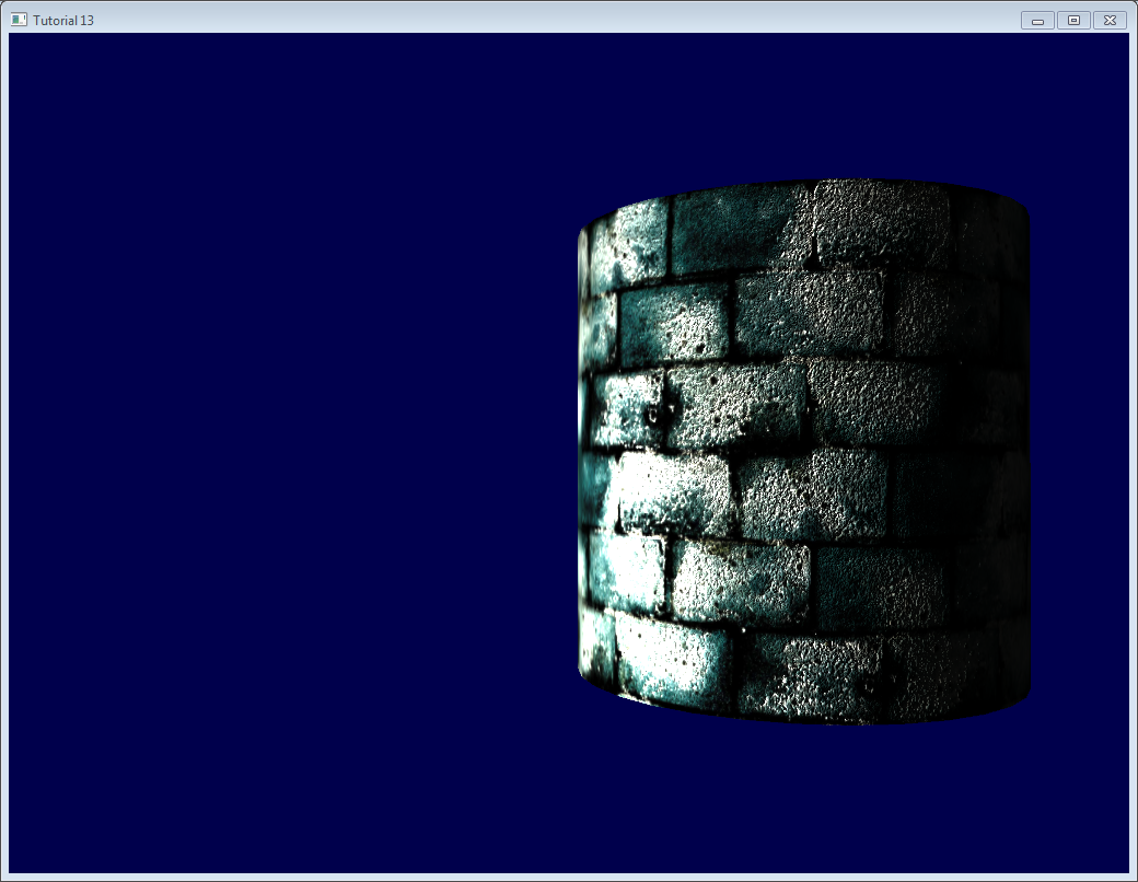
结果

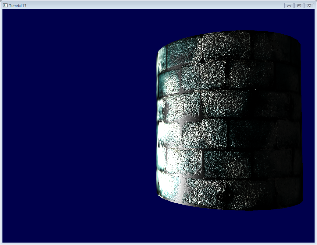
这是目前得到的结果，您可以看到：

• 砖块看上去凹凸不平，这是因为砖块表面法线变化比较剧烈
• 水泥部分看上去很平整，这是因为这部分的法线纹理全都是蓝色

延伸阅读

正交化（Orthogonalization）

顶点着色器中，为了计算速度，我们没有进行矩阵求逆，而是进行了转置。这只有当矩阵表示的空间正交时才成立，而这个矩阵还不是正交的。好在这个问题很容易解决：只需在computeTangentBasis()末尾让切线与法线垂直。

t = glm::normalize(t - n * glm::dot(n, t));

这个公式有点难理解，来看看图：

n和t差不多是相互垂直的，只要把t沿-n方向稍微“推”一下，幅度是dot(n,t)。
这里有一个applet也演示得很清楚（仅含两个向量）。

左手系还是右手系？

一般不必担心这个问题。但在某些情况下，比如使用对称模型时，UV坐标方向会出错，导致切线T方向错误。

判断是否需要翻转坐标系很容易：TBN必须形成一个右手坐标系——向量cross(n,t)应该和b同向。

用数学术语讲，“向量A和向量B同向”则有“dot(A,B)>0”；故只需检查dot( cross(n,t) , b )是否大于0。

若dot( cross(n,t) , b ) < 0，就要翻转t：

if (glm::dot(glm::cross(n, t), b) < 0.0f){
    t = t * -1.0f;
 }

在computeTangentBasis()末对每个顶点都做这个操作。

镜面纹理（Specular texture）

为了增强趣味性，我在代码里加上了镜面纹理；取代了原先作为镜面颜色的灰色vec3(0.3,0.3,0.3)。镜面纹理看起来像这样：

请注意，由于如上镜面纹理中没有镜面分量，水泥部分均呈黑色。

用立即模式（immediate mode）进行调试

本站的初衷是让大家不再使用已被废弃、缓慢、问题频出的立即模式。

不过，用立即模式进行调试却十分方便：

这里，我们在立即模式下画了一些线条表示切线空间。

要进入立即模式，必须先关闭3.3 Core Profile：

glfwOpenWindowHint(GLFW_OPENGL_PROFILE, GLFW_OPENGL_COMPAT_PROFILE);

然后把矩阵传给旧式的OpenGL流水线（你也可以另写一个着色器，不过这样做更简单，反正都是在hacking）：

glMatrixMode(GL_PROJECTION);
glLoadMatrixf((const GLfloat*)&ProjectionMatrix[0]);
glMatrixMode(GL_MODELVIEW);
glm::mat4 MV = ViewMatrix * ModelMatrix;
glLoadMatrixf((const GLfloat*)&MV[0]);

禁用着色器：

glUseProgram(0);

然后绘制线条（本例中法线都已被归一化，乘以0.1，置于对应顶点上）：

glColor3f(0,0,1);
glBegin(GL_LINES);
for (int i=0; i<indices.size(); i++){
    glm::vec3 p = indexed_vertices[indices[i]];
    glVertex3fv(&p.x);
    glm::vec3 o = glm::normalize(indexed_normals[indices[i]]);
    p+=o*0.1f;
    glVertex3fv(&p.x);
}
glEnd();

切记：实际项目中不要用立即模式！仅限调试时使用！别忘了之后恢复到Core Profile，它可以保证不启用立即模式！

利用颜色进行调试

调试时，将向量的值可视化很有用处。最简单的方法是把向量都写到帧缓冲。举个例子，我们把LightDirection_tangentspace可视化一下试试：

color.xyz = LightDirection_tangentspace;

这说明：

• 在圆柱体的右侧，光线（如白色线条所示）是朝上（在切线空间中）的。也就是说，光线和三角形的法线同向。

• 在圆柱体的中间部分，光线和切线方向（指向+X）同向。

一些提示：

• 可视化前，变量是否需要归一化取决于具体情况。
• 如果结果不易理解，就逐个分量可视化。比如，只观察红色，而将绿色和蓝色分量强制设为0。
• alpha值过于复杂，别折腾:)
• 若想将一个负值可视化，可以采用和处理法线纹理一样的技巧：转而把(v+1.0)/2.0可视化，于是黑色就代表-1，而白色代表+1。只不过这样做会让结果不直观。

利用变量名进行调试

前面已经讲过了，搞清楚向量所处的空间是关键。千万别用摄像机空间里的向量点乘模型空间里的向量。

给向量名称添加“_modelspace”后缀可以有效地避免这类计算错误。

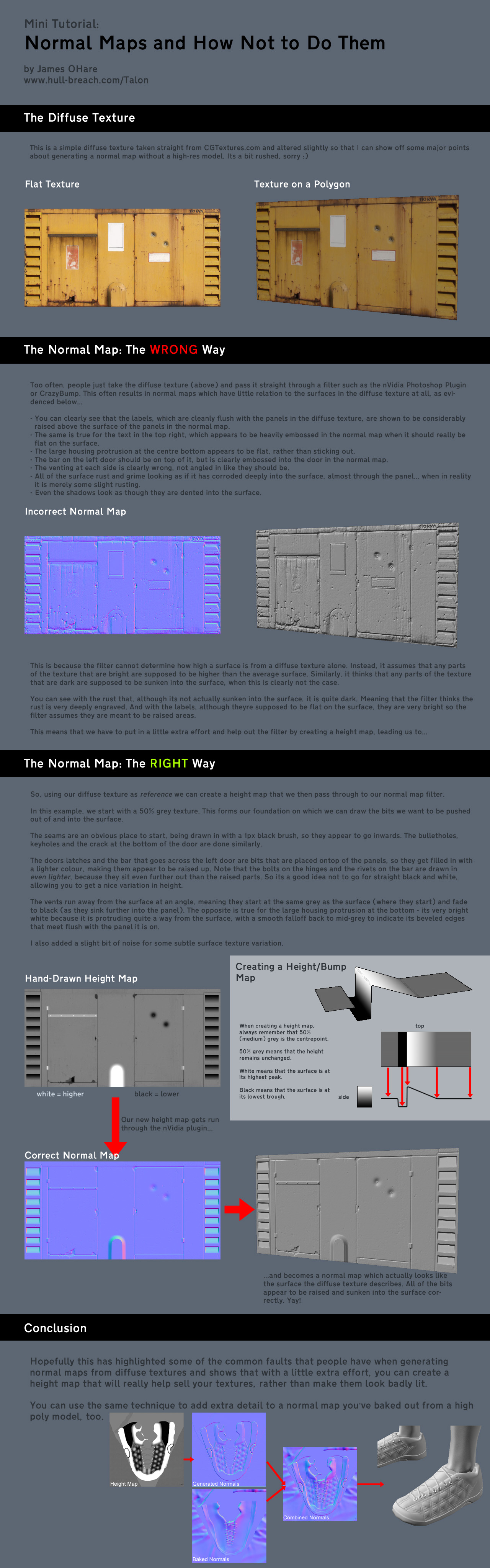
怎样制作法线贴图

作者James O’Hare。点击图片放大。

练习

• 在indexVBO_TBN函数中，做加法前先把向量归一化，观察其作用。
• 用颜色可视化其他向量（如instance、EyeDirection_tangentspace），试着解释您看到的结果。

工具和链接

• Crazybump 制作法线纹理的好工具，付费。
• Nvidia photoshop插件免费，不过Photoshop不免费……
• 用多幅照片制作法线贴图
• 用单幅照片制作法线贴图
• 关于矩阵转置的详细资料

参考文献

• Lengyel, Eric. “Computing Tangent Space Basis Vectors for an Arbitrary Mesh”. Terathon Software 3D Graphics Library, 2001.
• Real Time Rendering, third edition
• ShaderX4

© http://www.opengl-tutorial.org/

Written with Cmd Markdown.