期末作业 Random Systems

Abstract

Some of our systems of study is deterministic.Given some initial conditions,the motion of the projectile is completely determined, that is predictiable, for all future times.

Other system is random system. It can also be called stochastic systems.

Background

Take coffee and a drop of cream as an example. We make a cup of black coffee and delicately place a drop of cream at the center. The cream particles undergoes a complicated trajectory. We need statistical description and theory to study these system because we don't have to know all information of every particles but the average properties.
Each cream particle follows a complicated trajectory as it collides repeatedly with other particles. Such a trajectory can be modelled by what is known as a "random walk". This is a process in which a particle moves one step at a time, according to certain rules.

Main body

code1

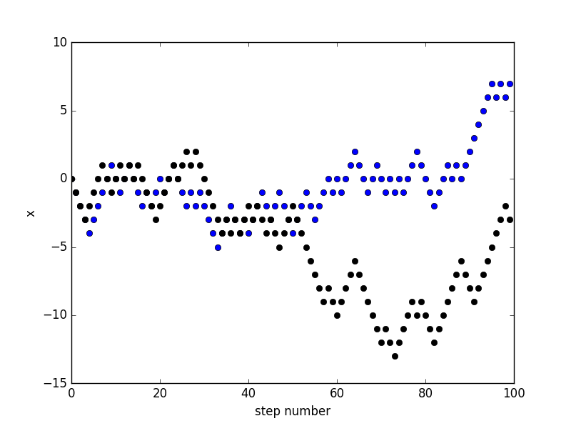
According to $<x^2>=2Dt$
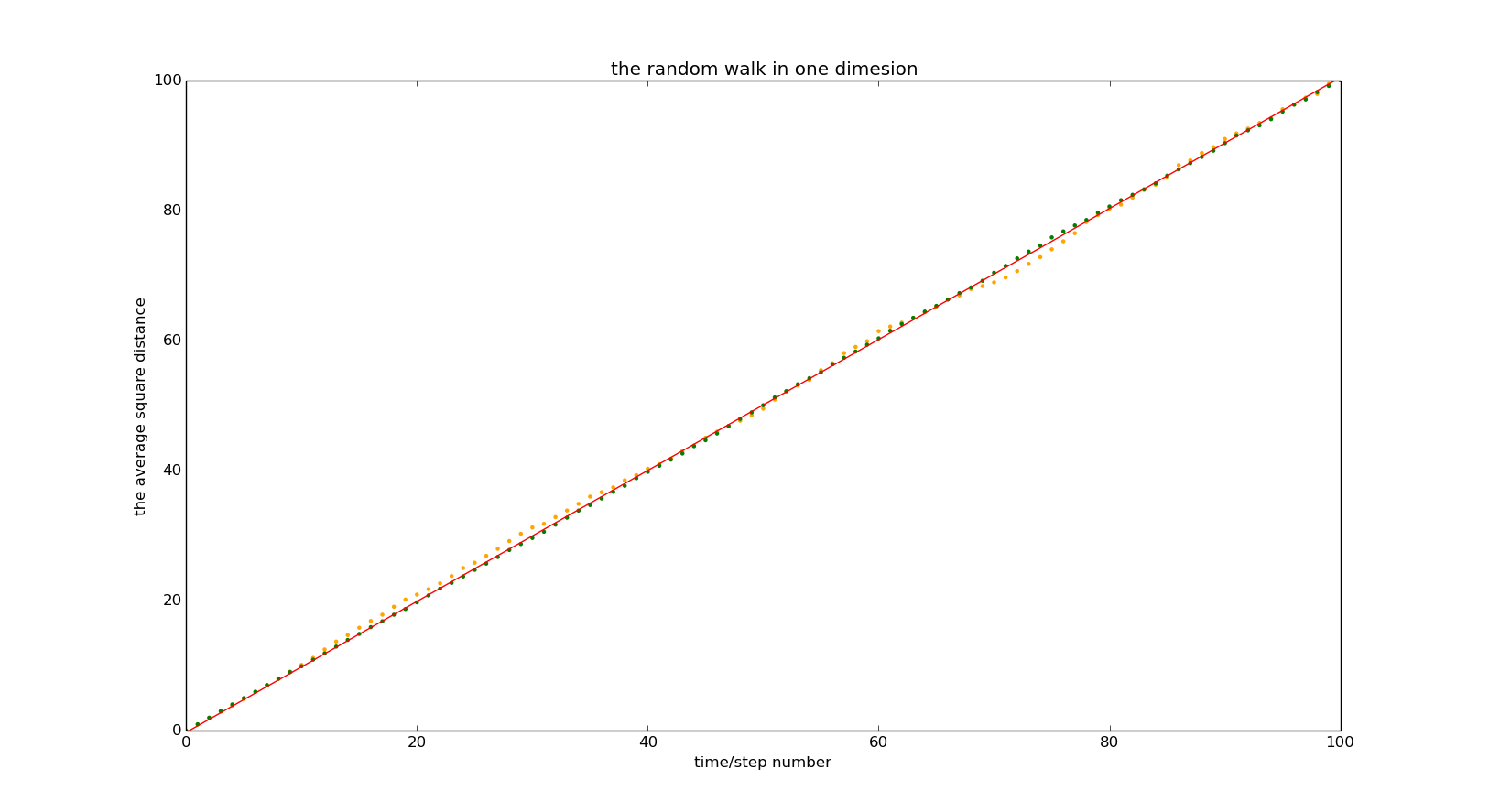
There are two points in the figure. The green average was 20,000, and the orange average was 2,000. We can say that there are some fluctuations in orange spots, but this is shown when the average sample size becomes larger. The fitted line is y = 1.004 * x-0.0337. Therefore, the $D$ value is 0.502.

In order to study the shape of macromolecules, it is linear, but can not intersect, which means that in a position can only be occupied once. We only study 2D SAW. In this case, we design a SAW model in which the path of a randomly wandering particle will not pass through the position it had previously passed. To accomplish this, we must scan the position of the previous step to see if it occupies four positions adjacent to the current particle position. If some are already occupied, the particles can not pass through them now.
There are two ways to achieve this goal: one is the simulation, the other is the enumeration. The simulation first generates a number of random walk paths, and if it has self-intersected and then discarded them, the rest can be all SAW paths. Enumeration is a step-by-step listing of possible SAW paths.
code2

For the simulation method, more than 200 SAW paths are finally obtained in step 50 and the average squared distance is obtained. Because of the relationship: $<r^2>=At^{2v}$ , we check the exact value of v.

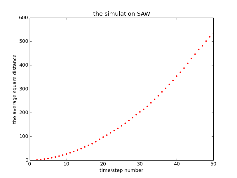
Here, we make a logarithmic-logarithmic fit to the equation. The resulting value of v is: 0.94462. This result is somewhat biased against the textbook result, and I get a value greater than the textbook, which I think leads to a value greater than the standard value of 0.75.

There are two ways to achieve this goal: one is the simulation, the other is the enumeration. The simulation first generates a number of random walk paths, and if it has self-intersected and then discarded them, the rest can be all SAW paths. Enumeration is a step-by-step listing of possible SAW paths.

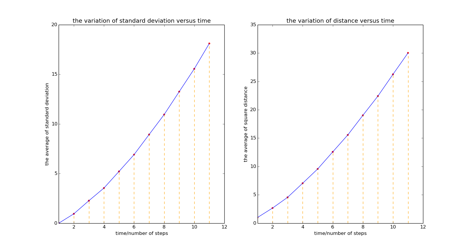
This is achieved by gradually averaging all possible SAW paths.

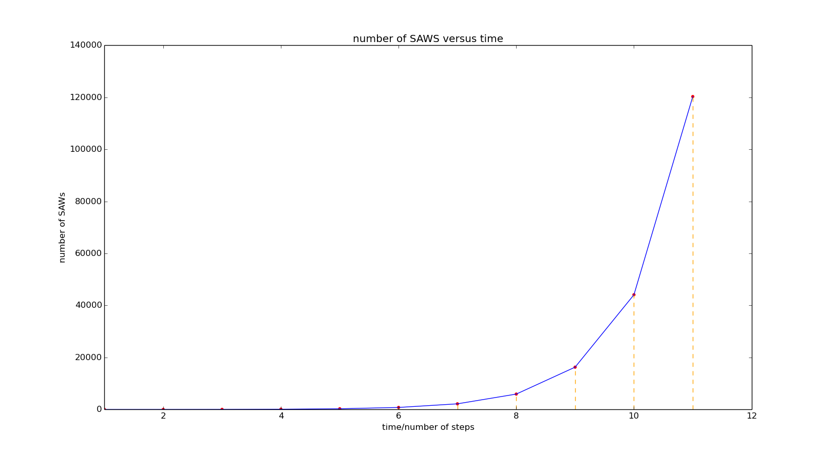
The number of possible SAW path increase rapidly versus time and that is the reason for I only do 11 steps. Again, due to the relation

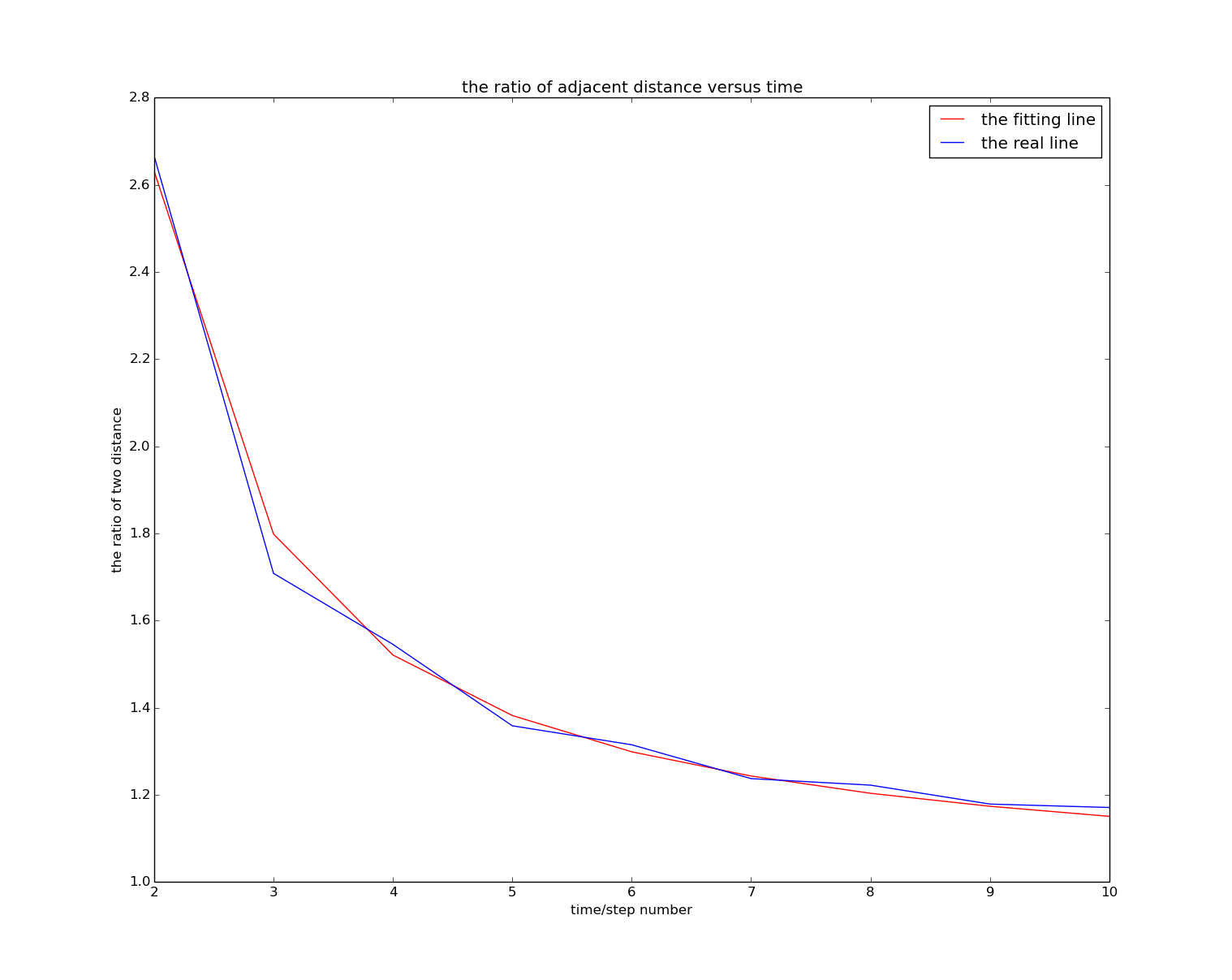
code3
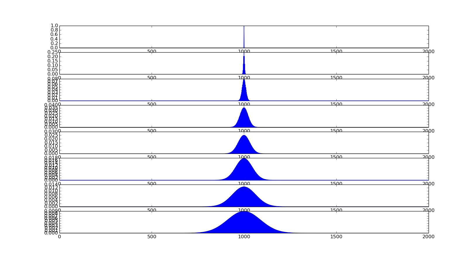
In the center set a sharp Gaussian as the initial condition, and then we can see the time evolution. We set $D=1.0$

Now let's see randomness in two dimensions again. We draw a picture that shows that if we comtain 200 random numbers for four times, the results don't relate to each other.

Conclusion

• By statistical description and theory, we understand the random system better.
• Several random walk systems have been studied, and it can be seen that it is a good approximation for many similar systems.
• For a while it revealed the nature of this system. However, it is important to note that particle interactions can not normally be ignored in practical systems. There is no doubt that in these factors are added to the simulation, the results will attract the reality, but this will also bring huge computational burden.

Acknowledgement

• Computational Physics, Nicholas J. Giordano & Hisao Nakanishi
• Think Python: How to Think Like a Computer Scientist, Allen B. Downey