Exercise_07 : Oscillatory and Motion and Chaos

Abstract

Write a program to calculate and compare the behavior of two, nearly identical pendulums. Use it to calculate the divergence of two nearby trajectories in the chaotic regime, as in Figure 3.7, and make a qualitative estimate of the corresponding Lyapunov exponent from the slope of a plot of $log(\Delta\theta)$ as a function of $t$ .

• use Euler-Cromer method to solve the oscillatory motion
• understand the chaos in the driven nonlinear pendulum.

Background

混沌是指现实世界中存在的一种貌似无规律的复杂运动形态。共同特征是原来遵循简单物理规律的有序运动形态，在某种条件下突然偏离预期的规律性而变成了无序的形态。混沌可在相当广泛的一些确定性动力学系统中发生。混沌在统计特性上类似于随机过程，被认为是确定性系统中的一种内禀随机性。

Main body

We first consider a nonlinear, damped, driven pendulum, the physical pendulum.
I choose the parameters are the same as the book :
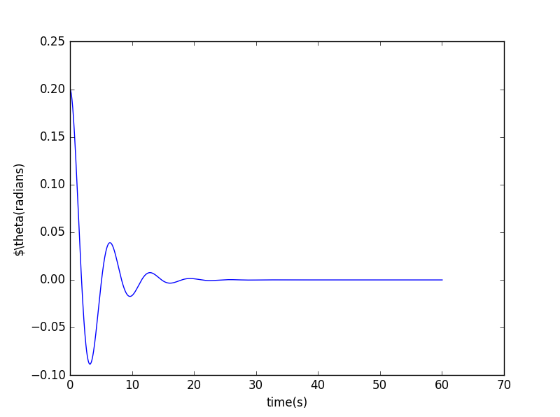
$q=0.5$ , $l=g=9.8$ , $\Omega_D=2/3$ , and $dt=0.04$
The initial conditions are $\theta(0)=0.2$ and $\omega(0)=0$ .

import pylab as pl
import math
class pendulum:
    def __init__(self, init_theta=0.2, init_omega=0,\
    length=9.8, g=9.8, time_step=0.04, q=0.5,fd=1.2, omega_d=2.0/3):
        self.w = [init_omega]
        self.theta = [init_theta]
        self.t = [0]
        self.dt = time_step
        self.g=g
        self.l=length
        self.q=q
        self.fd=fd
        self.omega_d=omega_d
    def run(self):
        while self.t[-1] < 60:
            self.w.append(self.w[-1] + (-self.g/ self.l * math.sin(self.theta[-1]) \
            -self.q * self.w[-1] + self.fd * math.sin(self.omega_d * self.t[-1])) *\
            self.dt)
            self.theta.append(self.theta[-1] + self.dt * self.w[-1])
            if self.theta[-1]> math.pi  :
                self.theta[-1]=self.theta[-1] - 2*math.pi
            if self.theta[-1]< -math.pi :
                self.theta[-1]=self.theta[-1] + 2*math.pi
            self.t.append(self.t[-1] + self.dt)
    def show_results(self):
        pl.plot(self.t, self.theta)
        pl.xlabel('time(s)')
        pl.ylabel(r'$\theta(radians)')
        pl.show()
a = pendulum()
a.run()
a.show_results()

when $F_D=0$:

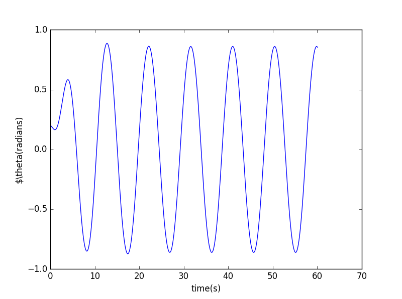
when $F_D=0.5$:

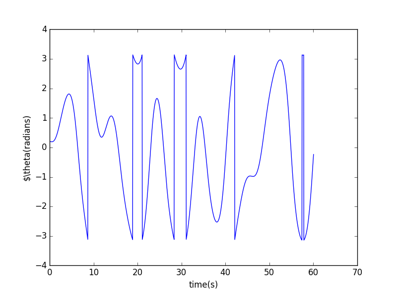
when $F_D=1.2$:

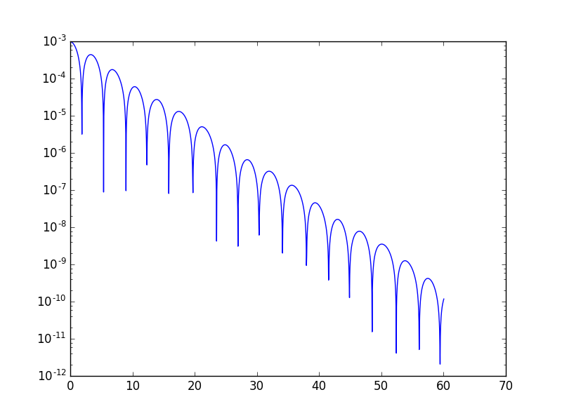
Then we consider the stability of the solution to our pendulum equation of motion. The only difference is that we start them with slightly different initial angles.

import pylab as pl
import math
class pendulum:
    def __init__(self, init_theta1=0.2, init_omega=0,init_theta2=0.201,\
        length=9.8, g=9.8, time_step=0.04, q=0.5,fd=1.2, omega_d=2.0/3):
        self.w1 = [init_omega]
        self.theta1 = [init_theta1]
        self.w2 = [init_omega]
        self.theta2 = [init_theta2]
        self.t = [0]
        self.dt = time_step
        self.g=g
        self.l=length
        self.q=q
        self.fd=fd
        self.omega_d=omega_d
        self.delta=[0]
    def run(self):
        while self.t[-1] < 60:
            self.w1.append(self.w1[-1] + (-self.g/ self.l * math.sin(self.theta1[-1]) \
            -self.q * self.w1[-1] + self.fd * math.sin(self.omega_d * self.t[-1])) *\
            self.dt)
            self.theta1.append(self.theta1[-1] + self.dt * self.w1[-1])
            #theta1
            self.w2.append(self.w2[-1] + (-self.g/ self.l * math.sin(self.theta2[-1]) \
            -self.q * self.w2[-1] + self.fd * math.sin(self.omega_d * self.t[-1])) *\
            self.dt)
            self.theta2.append(self.theta2[-1] + self.dt * self.w2[-1])
            #theta2
            self.t.append(self.t[-1] + self.dt)
            self.delta.append ( abs(self.theta1[-1]-self.theta2[-1]))
    def show_results(self):
        font = {'family': 'serif',
                'color':  'darkred',
                'weight': 'normal',
                'size': 16,}
        pl.semilogy(self.t,self.delta)
        pl.semilogy(self.t,self.e,'--')
        pl.title(r'$\Delta\theta$ versus time', fontdict = font)
        pl.xlabel('time(s)')
        pl.ylabel(r'$\Delta\theta$(radians)')
        pl.legend((['$F_D$=0.5']))
        pl.show()
a = pendulum()
a.run()
a.show_results()

When $F_D=0.5$

When $F_D=1.2$

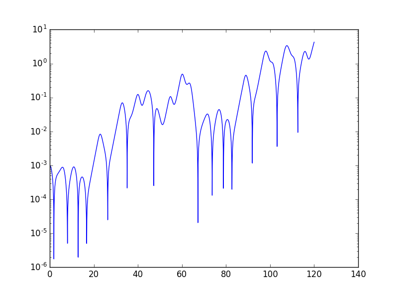
Conclusion

• We can see that at low drive the motion is a simple osciallation (after the transients have decayed). On the other hand, at high drive the motion is unstable. So we conclude that at low drive the motion is stable and at high drive the motion is chaotic.

• It turns out that $\Delta\theta\approx e^{\lambda t}$.
  the parameter $\lambda$ is known as Lyapunov exponent.
  In the former case $\lambda<0$ , in the latter case $\lambda>0$.

• Chaotic means a system can obey certain deterministic laws of physics, but still exhibit behavior that is unpredictable due to an extreme sensitivity to initial conditions.

Acknowledgement

Thanks to The Compulational Physics book.