Exercise 09:the Lorentz model

未分类

Abstract

• understand the chaos in the lorentz model by solving this set of ODE numerically. Building model to deal with the extending billiard problem with various boundary shape.

Background

Lorentz was studying the basic equations of fluid mechanics, which are known as the Navier-Stokes equations and which can be regarded as Newton’s law written in a form appropriate to a fluid. The specific situation he considered was the Rayleigh-Benard problem, which concerns a fluide in a container whose top and bottom surfaces are held at different temperatures. Indeed, he grossly simplified the problem as he reached to the so-called Lorentz equations, or equivalently, the Lorentz model, which provided a major contribution to the modern field of physics.

Main body

code

import matplotlib.pyplot as plt
from matplotlib import animation 
def loren(x0,y0,z0,r,sigma,b,dt,T):
    location=[[]for i in range(4)]
    location[0].append(x0)
    location[1].append(y0)
    location[2].append(z0)
    location[3].append(0)
    while location[3][-1]<=T:
        location[0].append(location[0][-1]+sigma*(location[1][-1]-location[0][-1])*dt)
        location[1].append(location[1][-1]+(-location[0][-2]*location[2][-1]+r*location[0][-2]-location[1][-1])*dt)
        location[2].append(location[2][-1]+(location[0][-2]*location[1][-2]-b*location[2][-1])*dt)
        location[3].append(location[3][-1]+dt)
    return location#x,y,z,time
sigma,b,dt,T=10,8./3,0.0001,50
d=loren(1,0,0,25,sigma,b,dt,T)
# first set up the figure, the axis, and the plot element we want to animate   
fig = plt.figure() 
ax = plt.axes(xlim=(-21, 21), ylim=(-1,45))
line, = ax.plot([], [],lw=1)  
plt.title('Fig. Lorentz Model')
plt.xlabel('x')
plt.ylabel('z')
note = ax.text(10,5,'',fontsize=12)
# initialization function: plot the background of each frame
def init():  
    line.set_data([], []) 
    note.set_text('') 
    return line,note
# animation function.  this is called sequentially   
def animate(j): 
    line.set_data(d[0][:1000*j],d[2][:1000*j]) 
    note.set_text(r'$x_0=1,y_0=0,z_0=0$'+'\n$\sigma=10,b=8/3,r=25$')
    return line,note
anim1=animation.FuncAnimation(fig, animate, init_func=init, frames=int(len(d[0])/1000), interval=10) 
#anim1.save('/home/shangguan/computationalphysics_N2013301020076/ex10/animr=25/haha.png')
plt.show()  

first is the phase gragh is the different regime(in this result we let the sigma equals to 10.0,b=8/3 and r=25.0)

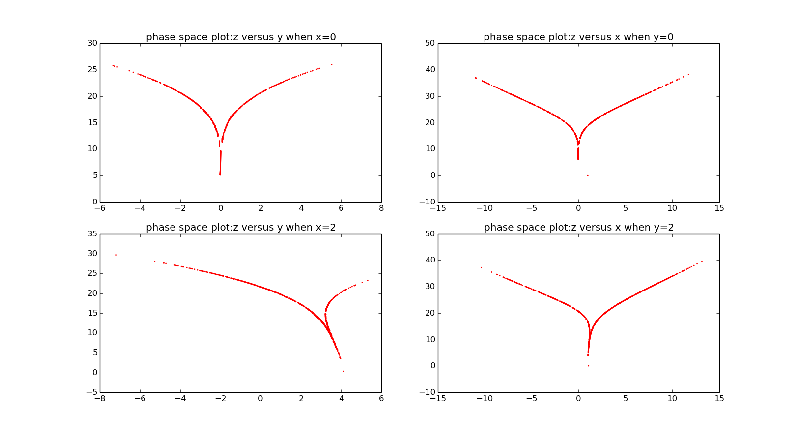
we can say the deviation of cross section of y-z is opposite to x-z.

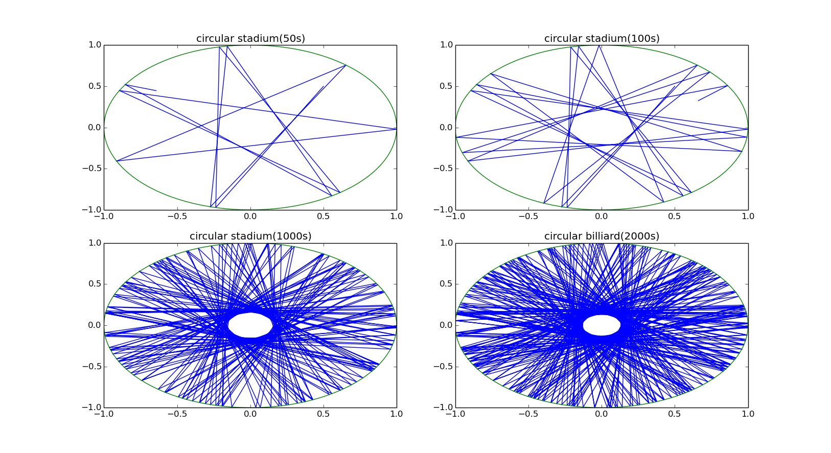
then we consider the circular stadium (r=1):

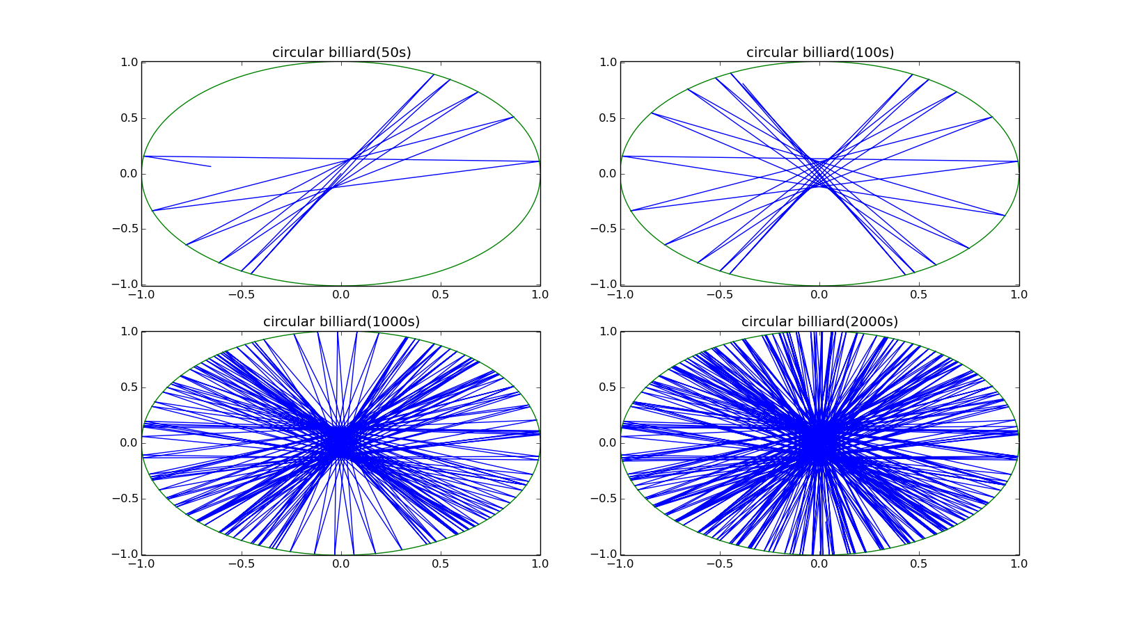
then the more realistic situation with a little separarion (r=1,l=0.02):

Acknowledgement

senior student
Computational Physics, Nicholas J. Giordano & Hisao Nakanishi