Exercise 08:Oscillatory and Motion and Chaos （2）

冯文龙

Abstract

Use python to study the oscillatory motion and chaos and complete the homework 3.18

Background

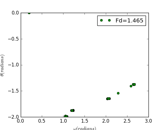
Poincare section Poincare section is preferred When we need to plot and analyse the behavior of a dynamical system. To construct Poincare section, we plot points only when the phases of the driven force are fixed, to be more specific, we plot $\omega$ only at times that are in phase with the driving force. The time can be determined by

$$\Omega_Dt=2n\pi$$ where n is an integer.

Bifurcation diagram helps to analyze the transition to chaos. It can show us lines for $\theta$ as a function of drive amplitude, which was constructed in the following manner. For each value of F_D we have calculated \theta as a function of time. After waiting for 300 driving periods so that the initial transients have decayed away, we plotted \theta at times that were in phase with the driving force as a function of F_D. Here we plotted points up to the 428th driving period. the Feigenbaum $\delta$ parameter can be calculate:

$$\delta_n=\frac{F_n-F_{n-1}}{F_{n+1}-F_n}$$

Main body

code:

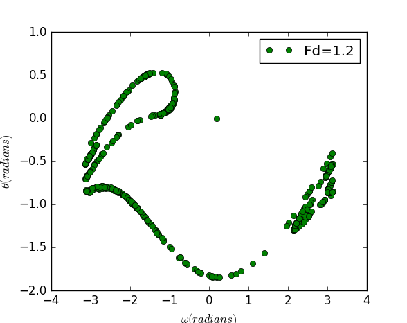
import pylab as pl
import math
class pendulum:
    def __init__(self, init_theta=0.2, init_omega=0,\
    length=9.8, g=9.8, time_step=0.04, q=0.5,fd=1.2, omega_d=2.0/3):
        self.w = [init_omega]
        self.theta = [init_theta]
        self.t = [0]
        self.dt = time_step
        self.g=g
        self.l=length
        self.q=q
        self.fd=fd
        self.omega_d=omega_d
        self.w_n=[init_omega]
        self.theta_n=[init_theta]
    def run(self):
        while self.t[-1] < 10000:
            self.w.append(self.w[-1] + (-self.g/ self.l * math.sin(self.theta[-1]) \
            -self.q * self.w[-1] + self.fd * math.sin(self.omega_d * self.t[-1])) *\
            self.dt)
            self.theta.append(self.theta[-1] + self.dt * self.w[-1])
            if self.theta[-1]> math.pi  :
                self.theta[-1]=self.theta[-1] - 2*math.pi
            if self.theta[-1]< -math.pi :
                self.theta[-1]=self.theta[-1] + 2*math.pi
            self.t.append(self.t[-1] + self.dt)
            if abs( self.t[-1]% (2 * math.pi /self.omega_d)) < self.dt /2:
                self.w_n.append(self.w[-1])
                self.theta_n.append(self.theta[-1])
    def show_results(self):
        pl.plot(self.theta_n, self.w_n,'go')
        pl.xlabel(r'$\omega(radians)$')
        pl.ylabel(r'$\theta(radians)$')
        pl.legend(['Fd=1.2'],loc="best")
        pl.show()
a = pendulum()
a.run()
a.show_results()

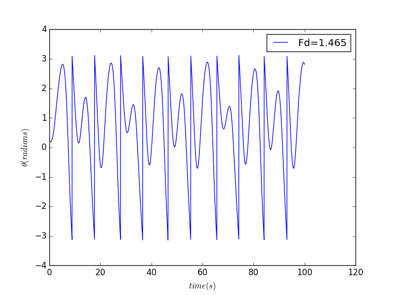
For $F_D=1.2$

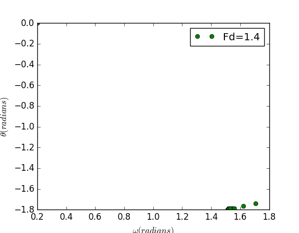
For $F_D=1.4$


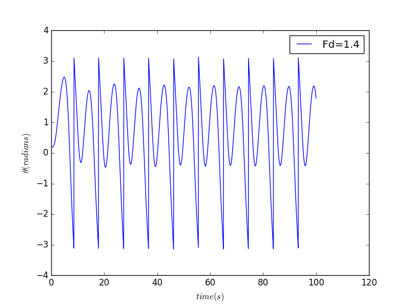
For$F_D=1.44$


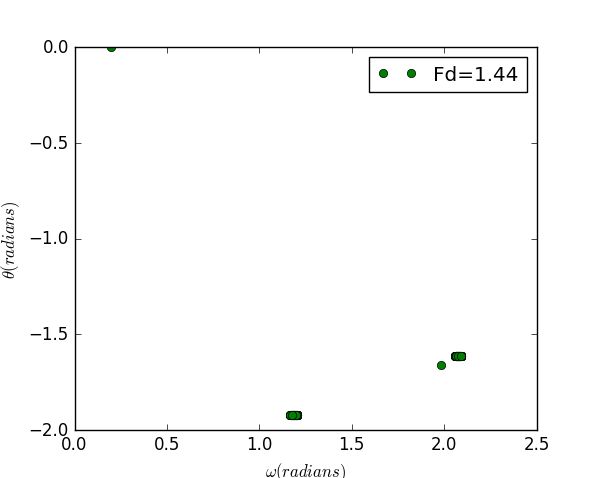
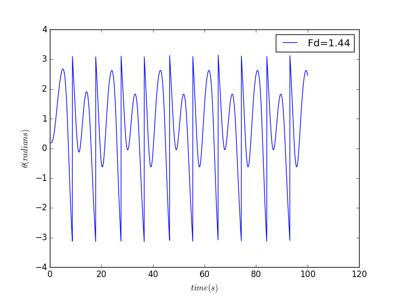
For$F_D=1.465$

Conclusion

• It turns out that the pendulum exhibits transitions to chaotic behavior at several different values of the driving force.
• when $F_D=1.4,1.44$ , we can see from the picture that the period is now twice the drive period. when $F_D=1.465$ , the period is four time the drive period.
• The key property is that it contains frequencies that are equal to or greater than the drive frequency.

Acknowledgement

Thanks to cai's PPT