Modelling and Visualization of High Dimensional Data

course

Curse of Dimensionality and Dimension Reduction

Facts:

• When the number of dimensions grows, the number of examples required to maintain a given sampling density grows exponentially.
• Humans have an extraordinary capacity to discern patterns and clusters in 1, 2 and 3-dimensions, but these capabilities degrade drastically for 4 or higher dimensions.

In practice, the curse of dimensionality means that, for a given sample size, there is a maximum number of features above which the performance of our classifier will degrade rather than improve:

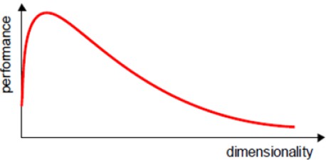
In most cases, the additional information that is lost by discarding some features is (more than) compensated by a more accurate mapping in the lower-dimensional space.

To conquer the curse of dimensionality, we often need dimension reduction. In fact, data in high dimensional space is not uniformly distributed. Often data is distributed in a lower dimension but presented in the high dimension. Recovering such a low-dimensional structure is a key to modelling high dimensional data in its very nature.

There are two methodologies of dimensionality reduction:

• Feature selection: choosing a subset of all the features.
• Feature extraction: creating a subset of new features by combinations.

However, reducing dimension leads to the problem of losing information.

PCA

Basic Algorithm

The goal of PCA (Principal Component Analysis) is to project the high-dimensional data onto a group of orthogonal unit vectors, where the variance of the projections is maximized. These vectors are called principal components.

Given a dataset of $N$ data points in a $d$-dimensional space, $\mathbf{X}=\{\mathbf{x}_1,\cdots,\mathbf{x}_N\}$.

• Subtract mean from data $\hat{\mathbf{x}}_n=\mathbf{x}_n-\bar{\mathbf{x}}$(where $\bar{\mathbf{x}}=\frac{1}{N}\sum_{n=1}^N\mathbf{x}_n$), denote the centralized data with $\hat{\mathbf{X}}=\{\hat{\mathbf{x}}_1,\cdots,\hat{\mathbf{x}}_N\}$.
• Define projection $z_n$ of centred data point $\hat{\mathbf{x}}_n$ onto unit length vector $\mathbf{u}$:

$$z_n=\mathbf{u}^T\hat{\mathbf{x}}_n$$

• Choose $\mathbf{u}$ to maximize variance of $\{z_1,\cdots,z_n\}$

$$var(\{z_1,\cdots,z_n\})=\frac{1}{N}\sum_{n=1}^N(z_n-\bar{z})^2$$

where $\bar{z}=\frac{1}{N}\sum_{n=1}^Nz_n$. Since $\hat{\mathbf{X}}$ is centralized, $\bar{z}=0$. Let $\mathbf{z}=[z_1\ \cdots\ z_N]^T$,

$$var(\{z_1,\cdots,z_n\})=\frac{1}{N}\sum_{n=1}^N(z_n)^2\\ =\frac{1}{N}\mathbf{z}\mathbf{z}^T\\ =\frac{1}{N}\mathbf{u}^T\hat{\mathbf{X}}\hat{\mathbf{X}}^T\mathbf{u}\\ =\mathbf{u}^T\mathbf{S}\mathbf{u}$$

where $\mathbf{S}=\frac{1}{N}\hat{\mathbf{X}}\hat{\mathbf{X}}^T=\frac{1}{N}\sum_{n=1}^N\hat{\mathbf{x}}_n\hat{\mathbf{x}}_n^T$ is the empirical covariance matrix. （or $\frac{1}{N-1}$ for unbiased estimation）

• Optimize Lagrangian imposing constraint $||\mathbf{u}||=\mathbf{u}^T\mathbf{u}=1$

$$\mathcal{L}(\mathbf{u})=\mathbf{u}^T\mathbf{S}\mathbf{u}+\lambda(1-\mathbf{u}^T\mathbf{u})$$

where $\lambda$ is the Lagrange multiplier.

• Setting the gradient w.r.t. $\mathbf{u}$ to zero gives optimality condition

$$\frac{\partial \mathcal{L}}{\partial \mathbf{u}}=2(\mathbf{S}\mathbf{u}-\lambda\mathbf{u})=0\\ \mathbf{S}\mathbf{u}=\lambda\mathbf{u}$$

• We say that $\mathbf{u}$ is an eigenvetor of $\mathbf{S}$ with eigenvalue $\lambda$.
• Multiplying by $\mathbf{u}$ on the left we get

$$\mathbf{u}^T\mathbf{S}\mathbf{u}=\lambda\mathbf{u}^T\mathbf{u}\\ var(\{z_1,\cdots,z_n\})=\lambda$$

so we should choose the eigenvector with the largest eigenvalue $\lambda$ as $\mathbf{u}$ to maximize the variance.

• The choice of $\mathbf{u}$ is the 1st principal component.
• To derive the 2nd principal component, define the projection $z'_n$ of the centred data $\hat{\mathbf{X}}$ onto another unit vector $\mathbf{u}'$

$$\mathbf{z}_n'=\mathbf{u}'\hat{\mathbf{x}}_n$$

Let $\mathbf{z}'=[z'_1\ \cdots\ z'_N]$. If $\mathbf{u}'$ is the 2nd principal component, it should follow the constraints that $\mathbf{u}$ and $\mathbf{u}'$ are orthogonal, i.e. $\mathbf{u}^T\mathbf{u}'=0$.

• $\mathbf{u}'$ is to maximize the variance of $\{z'_1,\cdots,z'_N\}$

$$var(\{z'_1,\cdots,z'_N\})=\frac{1}{N}\sum_{n=1}^N(z'_n)^2=\mathbf{u}'^T\mathbf{S}\mathbf{u}'$$

• Optimize Lagrangian imposing constraints

$$\mathcal{L}'(\mathbf{u}')=\mathbf{u}'^T\mathbf{S}\mathbf{u}'-\lambda'(1-\mathbf{u}'^T\mathbf{u}')-\phi\mathbf{u}^T\mathbf{u}'$$

where $\lambda'$ and $\phi$ are Lagrange multipliers.

• Setting the gradient w.r.t. $\mathbf{u}'$ to zero gives optimality condition

$$\frac{\partial \mathcal{L}'}{\partial \mathbf{u}'}=2\mathbf{S}\mathbf{u}'-2\lambda'\mathbf{u}'-\phi\mathbf{u}=0$$

By Multiplying $\mathbf{u}^T$ on the left, we get

$$2\mathbf{u}^T\mathbf{S}\mathbf{u}'-2\lambda'\mathbf{u}^T\mathbf{u}'-\phi\mathbf{u}^T\mathbf{u}=0$$

Note that

$$\mathbf{u}^T\mathbf{S}\mathbf{u}'=\mathbf{u}'^T\mathbf{S}\mathbf{u}=\mathbf{u}'^T\lambda\mathbf{u}=0$$

and

$$\mathbf{u}^T\mathbf{u}'=0$$

Therefore,

$$\phi=0\\ \mathbf{S}\mathbf{u}'-\lambda'\mathbf{u}'=0\\ \mathbf{S}\mathbf{u}'=\lambda'\mathbf{u}'$$

• $\mathbf{u}'$ is also an eigenvector of $\mathbf{S}$ with eigenvalue $\lambda'$.
• Multiplying by $\mathbf{u}'$ on the left we get

$$\mathbf{u}'^T\mathbf{S}\mathbf{u}'=\lambda'\mathbf{u}'^T\mathbf{u}'\\ var(\{z'_1,\cdots,z'_N\})=\lambda'$$

so we could choose the eigenvector with the second largest eigenvalue $\lambda$ as $\mathbf{u}'$ to maximize the variance. The choice of $\mathbf{u}'$ is the 2nd principal component.

• By repeating these steps, we could get the 3nd, 4th, ..., m-th principal components, which are the unit eigenvectors of $\mathbf{S}$ with the 3nd, 4th, ..., m-th largest eigenvalues.

Summary:

• For a given $d\times N$ dataset $\mathbf{X}$, subtracting the mean vector $\bar{\mathbf{X}}$ for all the instances in $\mathbf{X}$ to achieve the centralized dataset denoted by $\hat{\mathbf{X}}$.
• Calculate $\mathbf{S}=\frac{1}{N}\hat{\mathbf{X}}\hat{\mathbf{X}}^T$, finding out all $d$ eigenvalues, ranking them so that $\lambda_1\ge\cdots\lambda_d$, and their corresponing eigenvectors, $\mathbf{u}_1,\cdots,\mathbf{u}_d$.
• Selecting top $M$ ($M<d$) largest eigenvectors of $\mathbf{S}$ to form a project matrix $\mathbf{U}_M=[\mathbf{u}_1\ \mathbf{u}_2\ \cdots\ \mathbf{u}_M], \lambda_1\ge\cdots\lambda_M$.
• Encoding data point: $\mathbf{z}=\mathbf{U}_M^T(\mathbf{x}-\bar{\mathbf{x}})$, $\mathbf{z}$ is a $M$-dimensional vector encoding for the data point $\mathbf{x}$.
• Decoding (Reconstructing) data point: $\mathbf{x}'=\bar{\mathbf{x}}+\mathbf{U}_M\mathbf{z}$, $\mathbf{x}'$ is a $d$-dimensional vector for the data point $\mathbf{x}$.

Dual Algorithm

For a $d\times N$ ($d>>N$) matrix, $\mathbf{X}$, $\mathbf{S}=\frac{1}{N}\mathbf{X}\mathbf{X}^T$ is a $d\times d$ matrix. It is often computationally infeasible in solve its eigenvalue problem. We can construct a $N\times d$ matrix $\mathbf{Y}=\frac{1}{\sqrt{N}}\mathbf{X}^T$, which has

$$\mathbf{Y}^T\mathbf{Y}=\frac{1}{N}\mathbf{X}\mathbf{X}^T=\mathbf{S}$$

Then, we apply SVD (Singular Value Decomposition) on $\mathbf{Y}$

$$\mathbf{Y}=\mathbf{U}\mathbf{\Sigma}\mathbf{V}^T$$

Then transform $\mathbf{S}$ into

$$\mathbf{S}=\mathbf{Y}^T\mathbf{Y}=\mathbf{V}\mathbf{\Sigma}^T\mathbf{U}^T\mathbf{U}\mathbf{\Sigma}\mathbf{V}^T=\mathbf{V}\mathbf{\Sigma}^T\mathbf{\Sigma}\mathbf{V}^T$$

It is obvious to see that

$$\mathbf{S}\mathbf{V}=\mathbf{V}\mathbf{\Sigma}^T\mathbf{\Sigma}\mathbf{V}^T\mathbf{V}=\mathbf{V}\mathbf{\Sigma}^T\mathbf{\Sigma}$$

Since $\mathbf{\Sigma}$ is an diagonal matrix, the column vectors of $\mathbf{V}$ are eigenvectors of $\mathbf{S}$. Select first $M$ ($M < d$) columns of $\mathbf{V}$ (which is the first $M$ principal components) to form a project matrix $\mathbf{U}_M=[\mathbf{v}_1^T\ \cdots\ \mathbf{v}_M^T]$.

Summary:

• For a given $d\times N$ dataset $\mathbf{X}$, subtracting the mean vector $\bar{\mathbf{X}}$ for all the instances in $\mathbf{X}$ to achieve the centralized dataset denoted by $\hat{\mathbf{X}}$.
• Calculate $\mathbf{Y}=\frac{1}{\sqrt{N}}\mathbf{X}^T$ and apply SVD to $\mathbf{Y}$. Then we achieve a $d\times d$ matrix $\mathbf{V}^T$ (i.e., $\mathbf{Y}=\mathbf{U}\mathbf{\Sigma}\mathbf{V}^T$).
• Selecting first $M$ ($M < d$) columns of $\mathbf{V}$ to form a project matrix $\mathbf{U}_M=[\mathbf{v}_1^T\ \cdots\ \mathbf{v}_M^T]$.

Proportion of Variance

In practice, we can use Proportion of Variance (PoV) to determine an appropriate dimensionality $M$ in the PCA space:

$$PoV=\frac{\sum_{i=1}^k\lambda_i}{\sum_{i=1}^d\lambda_i}$$

When PoV >= 90%, the corresponding $k$ will be assigned to be $M$.

Limitations of the standard PCA

• The dimensions of maximum data variance are not always the relevant dimensions for preservation. (RCA, LDA, ...)
• Sometimes it is better to find independent rather than pair-wise uncorrelated/orthogonal dimensions. (ICA, ...)
• The reduction of dimensions for complex distributions may need nonlinear processing. (Nonlinear PCA extension)

LDA

Linear Discriminant Analysis (LDA) is a method for high-dimensional analysis in the supervised learning paradigm as class labels are available in a dataset. The objective of LDA is to perform dimensionality reduction while maximizing the difference between the projected means of different classes and minimizing the variance of projections of each class.

Two Classes

Assume we have a set of $d$-dimensional sample $\{\mathbf{x}_1,\cdots,\mathbf{x}_N\}$. $N_1$ of which belong to class $\omega_1$, and $N_2$ to class $\omega_2$. We seek to obtain a scalar $y$ by projecting the samples $\mathbf{x}$ onto a line $\mathbf{w}$

$$y=\mathbf{w}^T\mathbf{x}$$

The mean vector of each class in $\mathbf{x}$ and $y$ feature space is

$$\mu_i=\frac{1}{N_i}\sum_{\mathbf{x}\in\omega_i}\mathbf{x}\\ \tilde{\mu_i}=\frac{1}{N_i}\sum_{y\in\omega_i}y=\frac{1}{N_i}\sum_{\mathbf{x}\in\omega_i}\mathbf{w}^T\mathbf{x}=\mathbf{w}^T\mu_i$$

The difference between the projected means is

$$|\tilde{\mu_1}-\tilde{\mu_2}|^2=(\mathbf{w}^T\mu_1-\mathbf{w}^T\mu_2)^2\\ =\mathbf{w}^T(\mu_1-\mu_2)(\mu_1-\mu_2)^T\mathbf{w}\\ =\mathbf{w}^T\mathbf{S}_B\mathbf{w}$$

The matrix $\mathbf{S}_B$ is called the between-class scatter. Similarly, the variance of each class (called the scatter) is

$$\tilde{s_i}^2=\sum_{y\in\omega_i}(y-\tilde{\mu_i})^2=\mathbf{w}^T\mathbf{S}_i\mathbf{w}\\ \tilde{s_1}^2+\tilde{s_2}^2=\mathbf{w}^T\mathbf{S}_W\mathbf{w}$$

where

$$\mathbf{S}_i=\sum_{\mathbf{x}\in\omega_i}(\mathbf{x}-\mu_i)(\mathbf{x}-\mu_i)^T\\ \mathbf{S}_1+\mathbf{S}_2=\mathbf{S}_W$$

The matrix $\mathbf{S}_W$ is called the within-class scatter.

The criterion function (Fisher criterion) is defined as

$$J(\mathbf{w})=\frac{|\tilde{\mu_1}-\tilde{\mu_2}|^2}{\tilde{s_1}^2+\tilde{s_2}^2}=\frac{\mathbf{w}^T\mathbf{S}_B\mathbf{w}}{\mathbf{w}^T\mathbf{S}_W\mathbf{w}}$$

To find the maximum of $J(\mathbf{w})$, we derive and equate to zero

$$\frac{d}{d\mathbf{w}}[J(\mathbf{w})]=\frac{d}{d\mathbf{w}}[\frac{\mathbf{w}^T\mathbf{S}_B\mathbf{w}}{\mathbf{w}^T\mathbf{S}_W\mathbf{w}}]=0\Rightarrow\\ \frac{1}{\mathbf{w}^T\mathbf{S}_W\mathbf{w}}\frac{d[\mathbf{w}^T\mathbf{S}_B\mathbf{w}]}{d\mathbf{w}}-\frac{\mathbf{w}^T\mathbf{S}_B\mathbf{w}}{(\mathbf{w}^T\mathbf{S}_W\mathbf{w})^2}\frac{d[\mathbf{w}^T\mathbf{S}_W\mathbf{w}]}{d\mathbf{w}}=0\\ \frac{d[\mathbf{w}^T\mathbf{S}_B\mathbf{w}]}{d\mathbf{w}}-\frac{\mathbf{w}^T\mathbf{S}_B\mathbf{w}}{\mathbf{w}^T\mathbf{S}_W\mathbf{w}}\frac{d[\mathbf{w}^T\mathbf{S}_W\mathbf{w}]}{d\mathbf{w}}=0\Rightarrow\\ 2\mathbf{S}_B\mathbf{w}-\frac{\mathbf{w}^T\mathbf{S}_B\mathbf{w}}{\mathbf{w}^T\mathbf{S}_W\mathbf{w}}2\mathbf{S}_W\mathbf{w}=0\Rightarrow\\ \mathbf{S}_B\mathbf{w}-J(\mathbf{w})\mathbf{S}_W\mathbf{w}=0\Rightarrow\\ \mathbf{S}_W^{-1}\mathbf{S}_B\mathbf{w}-J(\mathbf{w})\mathbf{w}=0$$

$\mathbf{w}$ is an eigenvector of $\mathbf{S}_W^{-1}\mathbf{S}_B$.

$$\mathbf{S}_W^{-1}\mathbf{S}_B\mathbf{w}=J(\mathbf{w})\mathbf{w}\Rightarrow\\ \mathbf{S}_W^{-1}(\mu_1-\mu_2)(\mu_1-\mu_2)^T\mathbf{w}=J(\mathbf{w})\mathbf{w}$$

Note that $(\mu_1-\mu_2)^T\mathbf{w}$ and $J(\mathbf{W})$ are scalars, so $\mathbf{w}$ and $\mathbf{S}_W^{-1}(\mu_1-\mu_2)$ are in the same direction. As well, the scaling of $\mathbf{w}$ does not affect, so we can set

$$\mathbf{w}^*={\arg\max}_wJ(\mathbf{w})=\mathbf{S}_W^{-1}(\mu_1-\mu_2)$$

Summary:

• Estimate the within-class scatter matrix

$$\mathbf{S}_W=\sum_{i=1}^2\sum_{\mathbf{x}\in\omega_i}(\mathbf{x}-\mu_i)(\mathbf{x}-\mu_i)^T$$

where

$$\mu_i=\frac{1}{N_i}\sum_{\mathbf{x}\in\omega_i}\mathbf{x}$$

• Compute the optimal projection vector

$$\mathbf{w}=\mathbf{S}_W^{-1}(\mu_1-\mu_2)$$

• Apply the projection to samples

$$y=\mathbf{w}^T\mathbf{x}$$

Multiple Class

Denote the number of classes as $C$. LDA can only produce at most $C-1$ feature projections. The projection matrix $\mathbf{W}=[\mathbf{w}_1\ \cdots\ \ \mathbf{w}_{C-1}]$

$$\mathbf{y}=\mathbf{W}^T\mathbf{x}$$

The generalization of the within-class scatter is

$$\mathbf{S}_W=\sum_{i=1}^C\mathbf{S}_i$$

where $\mathbf{S}_i=\sum_{\mathbf{x}\in\omega_i}(\mathbf{x}-\mu_i)(\mathbf{x}-\mu_i)^T$ and $\mu_i=\frac{1}{N_i}\sum_{\mathbf{x}\in\omega_i}\mathbf{x}$

The generalization for the between-class scatter is

$$\mathbf{S}_B=\sum_i^CN_i(\mu_i-\mu)(\mu_i-\mu)^T$$

where $\mu=\frac{1}{N}\sum_{\forall\mathbf{x}}\mathbf{x}=\frac{1}{N}\sum_{i=1}^C\sum_{\mathbf{x}\in\omega_i}\mu_i=\frac{1}{N}\sum_{i=1}^CN_i\mu_i$

The total scatter matrix is defined as

$$\begin{array}{} \mathbf{S}_T=\sum_{\forall\mathbf{x}}(\mathbf{x}-\mu)(\mathbf{x}-\mu)^T\\ =\sum_{i=1}^C\sum_{\mathbf{x}\in\omega_i}(\mathbf{x}-\mu)(\mathbf{x}-\mu)^T\\ =\sum_{i=1}^C\sum_{\mathbf{x}\in\omega_i}(\mathbf{x}-\mu_i+\mu_i-\mu)(\mathbf{x}-\mu_i+\mu_i-\mu)^T\\ =\sum_{i=1}^C\sum_{\mathbf{x}\in\omega_i}[(\mathbf{x}-\mu_i)(\mathbf{x}-\mu_i)^T+(\mu_i-\mu)(\mu_i-\mu)^T+(\mathbf{x}-\mu_i)(\mu_i-\mu)^T+(\mu_i-\mu)(\mathbf{x}-\mu_i)^T]\\ =\mathbf{S}_B+\mathbf{S}_W+\sum_{i=1}^C\sum_{\mathbf{x}\in\omega_i}[(\mathbf{x}-\mu_i)(\mu_i-\mu)^T+(\mu_i-\mu)(\mathbf{x}-\mu_i)^T] \end{array}$$

Since $\mu_i=\frac{1}{N_i}\sum_{\mathbf{x}\in\omega_i}\mathbf{x}$, we can get

$$\sum_{i=1}^C\sum_{\mathbf{x}\in\omega_i}(\mathbf{x}-\mu_i)(\mu_i-\mu)^T\\ =\sum_{i=1}^C\left[\sum_{\mathbf{x}\in\omega_i}(\mathbf{x}-\mu_i)\right](\mu_i-\mu)^T\\ =\sum_{i=1}^C\left[N_i\mu_i-N_i\mu_i\right](\mu_i-\mu)^T=0$$

Similarly, we can get

$$\sum_{i=1}^C\sum_{\mathbf{x}\in\omega_i}(\mu_i-\mu)(\mathbf{x}-\mu_i)^T=0$$

Therefore,

$$\mathbf{S}_T=\sum_{\forall\mathbf{x}}(\mathbf{x}-\mu)(\mathbf{x}-\mu)^T=\mathbf{S}_B+\mathbf{S}_W$$

(However, $\mathbf{S}_T$ is not important is the algorithm of multiple class LDA. You can omit it)

Similarly, we define the mean vector and scatter matrices for the projected samples as

$$\tilde{\mu}_i=\frac{1}{N_i}\sum_{\mathbf{y}\in\omega_i}\mathbf{y}\\ \tilde{\mathbf{S}}_W=\sum_{i=1}^C\sum_{\mathbf{y}\in\omega_i}(\mathbf{y}-\tilde{\mu}_i)(\mathbf{y}-\tilde{\mu}_i)^T=\mathbf{W}^T\mathbf{S}_W\mathbf{W}\\ \tilde{\mu}=\frac{1}{N}\sum_{\forall\mathbf{y}}\mathbf{y}\\ \tilde{\mathbf{S}}_B=\sum_i^CN_i(\tilde{\mu}_i-\tilde{\mu})(\tilde{\mu}_i-\tilde{\mu})^T=\mathbf{W}^T\mathbf{S}_B\mathbf{W}$$

Since the projection is no long a scalar (it has $C-1$ dimensions), we then use the determinant of the scatter matrices to obtain a scalar objective function:

$$J(\mathbf{W})=\frac{|\tilde{\mathbf{S}}_B|}{|\tilde{\mathbf{S}}_W|}=\frac{|\mathbf{W}^T\mathbf{S}_B\mathbf{W}|}{|\mathbf{W}^T\mathbf{S}_W\mathbf{W}|}$$

It can be shown that the optimal projection matrix $\mathbf{W}^*$ is the one whose columns are the eigenvectors corresponding to the largest eigenvalues of the following generalized eigenvalue problem

$$\mathbf{W}^*=[\mathbf{w}_1^*\ \cdots\ \mathbf{w}_{C-1}^*]= {\arg\max}_{\mathbf{W}}\left\{\frac{|\mathbf{W}^T\mathbf{S}_B\mathbf{W}|}{|\mathbf{W}^T\mathbf{S}_W\mathbf{W}|}\right\}\\\Rightarrow \mathbf{S}_W^{-1}\mathbf{S}_B\mathbf{w}_i^*-\lambda_i\mathbf{w}_i^*=0$$

Note that in $\mathbf{S}_B=\sum_i^CN_i(\mu_i-\mu)(\mu_i-\mu)^T$, each $(\mu_i-\mu)(\mu_i-\mu)^T$ is the product of two vectors, so $\mathbf{S}_B$ is the sum of $C$ matrices of rank one or less, and therefore $rank(\mathbf{S}_B)\leq C$.

Ref: Rank Wiki. $Rank(AB)\leq\min(Rank(A),Rank(B))$, $Rank(A+B)\leq Rank(A)+Rank(B)$.

At the mean time, $\mu=\frac{1}{C}\sum_{i=1}^C\mu_i$, $(\mu_1-\mu),\cdots,(\mu_C-\mu)$ are linearly dependent, at least one $(\mu_i-\mu)$ could be represented by the others.

Note that $\mathbf{S}_B=\mathbf{M}\mathbf{N}\mathbf{M}^T$, where $\mathbf{N}=diag(N_1,\cdots,N_C)$, $\mathbf{M}=[(\mu_1-\mu)\ \cdots\ (\mu_C-\mu)]$. Therefore,

$$Rank(\mathbf{S}_B)\leq \min(Rank(\mathbf{M}),Rank(\mathbf{M}^T),Rank(\mathbf{N}))\\ =\min(C, r, r)$$

where $r$ is the rank of $\mathbf{M}$. Since it has at most $C-1$ linearly independent columns, its rank is at most $C-1$. Therefore, $Rank(\mathbf{S}_B)\leq C-1$. This means that at most $(C-1)$ of the eigenvalues $\lambda_i$ will be non-zero, and therefore LDA could reduce the samples to at most $(C-1)$ dimensions.

Summary:

• Estimate the within-class and between-class scatter scatter matrices

$$\mathbf{S}_W=\sum_{i=1}^C\sum_{\mathbf{x}\in\omega_i}(\mathbf{x}-\mu_i)(\mathbf{x}-\mu_i)^T$$

where $\mu_i=\frac{1}{N_i}\sum_{\mathbf{x}\in\omega_i}\mathbf{x}$

$$\mathbf{S}_B=\sum_i^CN_i(\mu_i-\mu)(\mu_i-\mu)^T$$

where $\mu=\frac{1}{N}\sum_{i=1}^CN_i\mu_i$

• Compute the optimal projection matrix $\mathbf{W}=[\mathbf{w}_1\ \cdots\ \mathbf{w}_{C-1}]$, where $\mathbf{w}_k$ is the k-th eigenvector of $\mathbf{S}_W^{-1}\mathbf{S}_B$.

• Apply the projection to samples

$$\mathbf{y}=\mathbf{W}^T\mathbf{x}$$

Limitations of LDA

• LDA produces at most $(C-1)$ feature projections.
• LDA is a parametric method since it assumes unimodal Gaussian likelihoods. If the distributions are significantly non-Gaussian, the LDA projections will not be able to preserve any complex structure of the data, which may be needed for classification.

SOM

Self-Organizing Map (SOM) is a biologically inspired unsupervised neural network that approximates an unlimited number of input data by a finite set of nodes arranged in a low-dimensional grid (one or two-dimensional), where neighbor nodes correspond to more similar input data.

Each neuron in a SOM (an one or two-dimensional grid) is assigned a weight vector with the same dimensionality $d$ as the input space (or, weight space). What we do is like updating these weights to make this grid "cover" all samples. The updating strategy is as following:

• Initialize weights randomly.
• For each sample, find the closest weight vector, and call the corresponding neuron winner (Best Matching Unit, BMU).
• "Pull" weights towards the sample. Weights of neurons that are closer to the winner (on the map space, which is one or two-dimensional. The distance between neurons is defined as the Manhattan distance of them on the grid and "neighborhood" is dtermined on the lattice topology) will adapt more heavily than neurons that are further away. The following figure shows an adaptation on two-dimensional weight space:

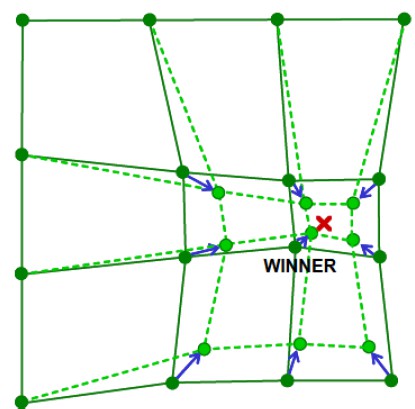
• After a number of iterations, the weights cover samples in an appropriate way. Note that during the iteration, we should decrease the learning rate and the neighborhood size (the parameter measures how much a neuron could affect other neurons) continuously to perform better training.

Summary:

• Initialize weights $\mathbf{w}_1, \cdots, \mathbf{w}_z$ to some small, random values. $z$ is the number of neurons.

• Repeat until convergence

  • Select the next input sample $\mathbf{x}_n$
  • Find the weight $\mathbf{w}_i$ that best matches $\mathbf{x}_n$. The corresponding neuron of $\mathbf{w}_i$ is the winner. The $d_E(\cdot)$ is the distance function.
  $$i={\arg\min}_{j}d_E(\mathbf{x}_n,\mathbf{w}_j)$$
  • Update the weights of the winner and all its neightbors $\mathbf{w}_k$
  $$\mathbf{w}_k=\mathbf{w}_k+\eta(t)\cdot h_{ik}(t)\cdot(\mathbf{x}_n-\mathbf{w}_k)$$

  where $\eta(t)$ is the learning rate related to the number of iteration $t$: $\eta(t)=\eta_0\exp(-\frac{t}{\tau_1})$. The $h_{ik}(t)=\exp(-\frac{d_{ik}^2}{2\sigma^2(t)})$ is the neighborhood kernel function, where $d_{ik}$ is the Manhattan distance between neurons $i$ and $k$ and $\sigma(t)=\sigma_0\exp(-\frac{t}{\tau_2})$ is the neighborhood size. $\eta_0,\tau_1,\tau_2,\sigma_0$ are hyper-parameters.

U-Matrix

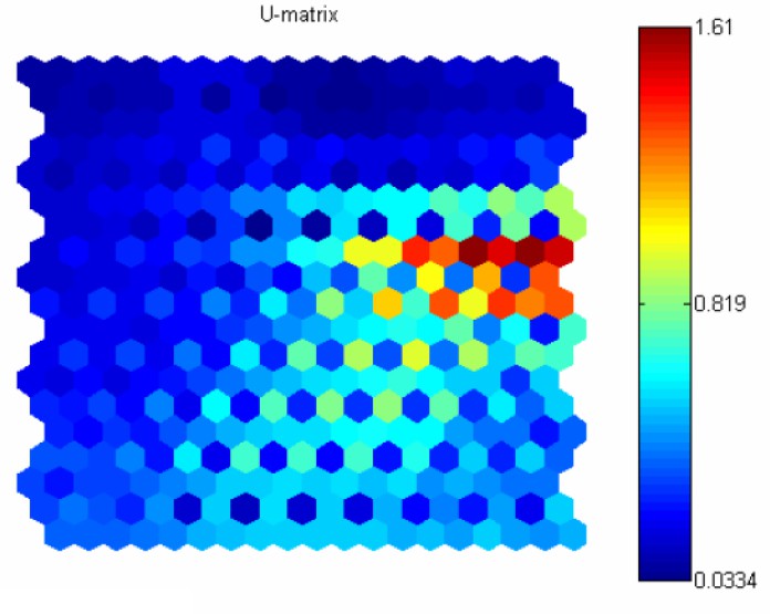
For weight space of dimension less than 4, neurons could be visualized by their corresponding weight vectors. For high-dimensional data, a unified distance matrix (U-matrix) is constructed to facilitate the visualization. The shape of one kind of U-matrix is the same as the SOM network. The corresponding value $U(i)$ in the U-matrix of the neuron $i$ is as the following:

$$U(i)=\frac{\sum_{k\in N(i)}d_E(\mathbf{w}_i, \mathbf{w}_k)}{|N(i)|}$$

where $N(i)$ is the set of neighbors of $i$. Distance between the weights of neighboring neurons gives an approximation of the distance between different parts of the underlying data. Dipict U-matrix in an image (heat map), similar colors depict the closely spaced nodes and distinct colors indicate the more distant nodes. Groups of similar colors can be considered as clusters, and the contrast parts as the boundary regions.

MDS

Multi-dimensional scaling (MDS) maps the distance between observations in a high dimensional space into a lower dimensional space. The goal is to find a configuration of points in the low dimensional space whose inter-point distance preserves dissimilarities of corresponding points in the higher dimension.

Iterative

Given points $\mathbf{x}_1,\cdots,\mathbf{x}_N$ in $d$ dimensions, the distance between points $\mathbf{x}_i$ and $\mathbf{x}_j$ is $\delta_{ij}$. We want to find points $\mathbf{y}_1,\cdots,\mathbf{y}_N$ in 2 (or 3) dimensions s.t. the distance $d_{ij}$ between $\mathbf{y}_i$ and $\mathbf{y}_j$ is close to $\delta_{ij}$. We can look for $d_{ij}$ by minimizing an objective function. The following are three possible objective functions (Stress):

$$J_{ee}=\frac{\sum_{i=1}^N\sum_{j>i}(d_{ij}-\delta_{ij})^2}{\sum_{i=1}^N\sum_{j>i}\delta_{ij}^2}\\ J_{ff}=\sum_{i=1}^N\sum_{j>i}\left(\frac{d_{ij}-\delta_{ij}}{\delta_{ij}}\right)^2\\ J_{ef}=\frac{1}{\sum_{i=1}^N\sum_{j>i}\delta_{ij}}\sum_{i=1}^N\sum_{j>i}\frac{(d_{ij}-\delta_{ij})^2}{\delta_{ij}}$$

Note that the $\delta_{ij}$s are constant. $J_{ee}$ penalizes large absolute errors. $J_{ff}$ penalizes large relative errors. $J_{ef}$ is a compromise between the two before.

For each low dimensional point $\mathbf{y}_k$, update it by:

$$\begin{array}{} \nabla J_{ee}(\mathbf{y}_k)=\frac{2}{\sum_{i=1}^N\sum_{j>i}\delta_{ij}^2}\sum_{j\not=k}(d_{kj}-\delta_{kj})\frac{\mathbf{y}_k-\mathbf{y}_j}{d_{kj}}\\ \nabla J_{ff}(\mathbf{y}_k)=2\sum_{j\not=k}\frac{d_{kj}-\delta_{kj}}{\delta_{kj}^2}\frac{\mathbf{y}_k-\mathbf{y}_j}{d_{kj}}\\ \nabla J_{ef}(\mathbf{y}_k)=\frac{2}{\sum_{i=1}^N\sum_{j>i}\delta_{ij}}\sum_{j\not=k}\frac{d_{kj}-\delta_{kj}}{\delta_{kj}}\frac{\mathbf{y}_k-\mathbf{y}_j}{d_{kj}} \end{array}$$

$$\mathbf{y}_k\leftarrow \mathbf{y}_k-\eta\nabla J(\mathbf{y}_k)$$

Summary:

• Determine the dimension of $\mathbf{y}_1,\cdots,\mathbf{y}_n$ and initialize them randomly.
• Calculate the distance of samples in the original space $\delta_{ij}$.
• Repeat:
  
  • Calculate the distance of samples in the target space $d_{ij}$, disparities (i.e. $d_{ij}-\delta_{ij}$) and the Stress.
  • If $Stress^{(t)}-Stress^{(t-1)}\ge\epsilon$, update each $\mathbf{y}$. Otherwise, break.

Analytic

Given the distance matrix $\delta_{ij}$ in the high dimensional space, denote the low dimensional embeddings as $\mathbf{Y}\in\mathbb{R}^{d'\times N}, d'<d$ and the low dimensional distance $d_{ij}=||\mathbf{y}_i-\mathbf{y}_j||$. It is expected that $d_{ij}=\delta_{ij}$. Therefore,

$$\delta_{ij}^2=||\mathbf{y}_i||^2+||\mathbf{y}_j||^2-2\mathbf{y}_i^T\mathbf{y}_j\\ =b_{ii}+b_{jj}-2b_{ij}$$

where the matrix $\mathbf{B}=\mathbf{Y}^T\mathbf{Y}\in\mathbb{R}^{m\times m}$ is the inner product matrix of embeddings. To simplify, we can centralize the embeddings $\mathbf{Y}$, i.e. $\sum_{i=1}^N\mathbf{y}_i=0$. Obviously, $\sum_{i=1}^Nb_{ij}=\sum_{j=1}^Nb_{ij}=0$. Therefore,

$$\sum_{i=1}^N\delta_{ij}^2=tr(\mathbf{B})+Nb_{jj}\\ \sum_{j=1}^N\delta_{ij}^2=tr(\mathbf{B})+Nb_{ii}\\ \sum_{i=1}^N\sum_{j=1}^N\delta_{ij}^2=2Ntr(\mathbf{B})$$

where $tr(\mathbf{B})$ is the trace of $\mathbf{B}$, i.e. $tr(\mathbf{B})=\sum_{i=1}^Nb_{ii}$. So, we can get

$$b_{ij}=-\frac{1}{2}(\delta_{ij}^2-\frac{1}{N}\sum_{j=1}^N\delta_{ij}^2-\frac{1}{N}\sum_{i=1}^N\delta_{ij}^2+\frac{1}{N^2}\sum_{i=1}^N\sum_{j=1}^N\delta_{ij}^2)$$

If we let $\mathbf{S}=\delta\odot\delta$, we can derive that $\mathbf{B}=-\frac{1}{2}\mathbf{H}\mathbf{S}\mathbf{H}$, where $\mathbf{H}=\mathbf{I}-\frac{1}{N}\mathbf{e}\mathbf{e}^T$ and $\mathbf{e}=[1\ 1\ \cdots\ 1]^T$.

After we derive the matrix $\mathbf{B}$, what we need next is to apply eigenvalue decomposition on $\mathbf{B}$: $\mathbf{B}=\mathbf{V}\mathbf{\Lambda}\mathbf{V}^T$. Suppose there are $d^*$ non-zero eigenvalues $\lambda_1 \ge \lambda_2\ge\cdots\ge\lambda_{d^*}$ in $\mathbf{\Lambda}$, they form the diagnoal matrix $\mathbf{\Lambda}_*=diag(\lambda_1,\cdots,\lambda_{d^*})$, and let $\mathbf{V}_*$ denotes the corresponding eigenvectors, then $\mathbf{Y}$ can be represented as:

$$\mathbf{Y}=\mathbf{\Lambda}_*^{1/2}\mathbf{V}_*^T\in\mathbb{R}^{d^*\times N}$$

If we do not need $\delta_{ij}=d_{ij}$ strictly and expect to reduce dimensionality effectively, we can select a $d'<d^*$ to construct $\mathbf{Y}$.

Summary:

• Get the distance matrix $\delta$ in the high dimensional space.
• Compute the inner product matrix $\mathbf{B}$.
• Apply eigenvalue decomposition on $\mathbf{B}$.
• Select $d'$ biggest eigenvalues $\tilde{\mathbf{\Lambda}}$ and corresponding eigenvectors $\tilde{\mathbf{V}}$ to construct the low dimensional embeddings $\mathbf{Y}=\tilde{\mathbf{\Lambda}}^{1/2}\tilde{\mathbf{V}}^T\in\mathbb{R}^{d'\times N}$.

MDS Family

• Metric-based MDS algorithms differ in
  
  • Dissimilarity (distance) or similarity metrics in high dimensional space.
  • Stress (objective) functions.
  • Optimization procedure. The linear MDS are analytic solvable but cannot model complex (nonlinear) low dimensional manifold well. The nonlinear MDS often needs to use an iterative algorithm (e.g. Gradient Descent).
  • The Nonmetric MDS (nMDS) only maintains the same ranking order in the low dimensional space as those in the high dimensional space.

ISOMAP

Isometric feature mapping (ISOMAP) is a non-linear MDS method for modelling manifold structure appearing in a high dimensional space. The ISOMAP preserves the geodesic distances between points, while the (normal) MDS preserves the Euclidean distances.

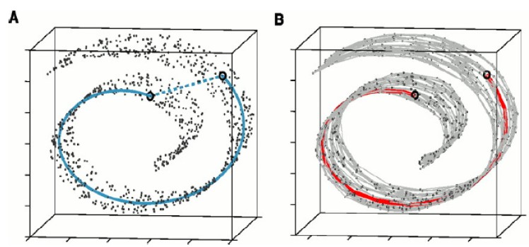
(The left figure depicts the Euclidean distance of two points, while the right figure depicts the geodesic distance between them (the red line))

For neighboring samples, the Euclidean distance provides a good approximation to geodesic distance. For distant points, the geodesic distance can be approximated with a sequence of steps between clusters of neighboring points. Therefore, the first step of the algorithm is to determine which points are neighbors in the manifold, based on the distance $d_X(i,j)$ in the input space $X$. The set of neighbors can be determined in two different ways:

• Connect each point to all points within a fixed radius $\epsilon$.
• Connect each point to all of its $K$ nearest neighbors.

The first method may cause problems if the samples are sparse. The second one might be affected by outliers. These neighborhood relations are represented as a weighted graph $G$. Then, we can estimate the geodesic distances $d_M(i,j)$ between all pair of points on the maniford $M$ by computing their shortest path distances $d_G(i,j)$ in the graph $G$. This can be performed, e.g. using Dijkstra's Algorithm, Floyd–Warshall algorithm. The distance matrix $D_G=\{d_G(i,j)\}$ is then inputted to the classical MDS algorithm (analytical solution).

Summary:

• Construct a neighborhood graph and compute the distance matrix $\delta$ (shortest path).
• Apply classical MDS algorithm to construct the low-dimensional embeddings $\mathbf{Y}$.

Limitations of ISOMAP

• ISOMAP is guaranteed asymptotically to recover the true dimensionality and geometric structure of manifolds whose intrinsic geometry is that of a convex region of Euclidean space, but it may fail if the intrinsic parameter space is not convex.
• Points need to be sampled uniformly (densely) from a noiseless manifold to do geodesic approximation.
• There might not exist an isometric emdedding (i.e. the output of MDS might not be ideal).
• Suffer from a high computational cost and sensitive to noise.
• ISOMAP does not provide a mapping function $\mathbf{Y}=f(\mathbf{X})$.

LLE

Locally Linear Embedding (LLE) is another non-linear method for modelling manifold structure. It models the local geometry of samples in the high dimensional space, and expects that after projecting to the low dimensional space they can keep the local geometry. The local geometry is modeled by linear weights that reconstruct each data point as a linear combination of its neighbors.

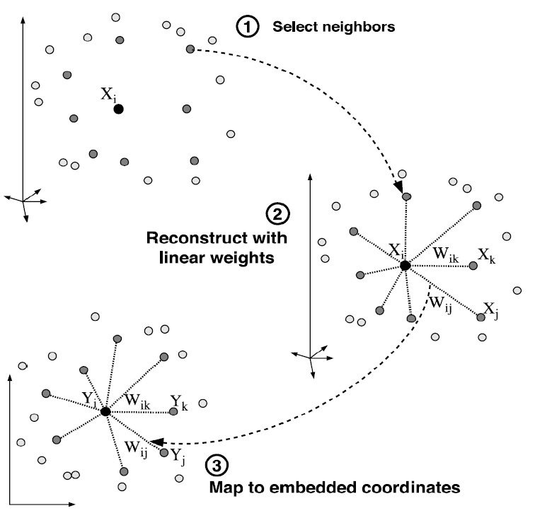
For each points

$$\mathbf{x}_i=\sum_{j=1}^Nw_{ij}\mathbf{x}_j\\ \text{s.t.}\sum_{j=1}^Nw_{ij}=1.$$

where the weight $w_{ij}$ measures the contribution of the j-th sample to the reconstruction of the i-th sample. If $\mathbf{x}_j$ is not the neighbor of $\mathbf{x}_i$, $w_{ij}=0$. These weights are computed by minimizing the reconstruction error

$$\min_{w}\sum_{i=1}^N||\mathbf{x}_i-\sum_{j=1}^Nw_{ij}\mathbf{x}_j||^2$$

The reconstruction error is equivalent to

$$\begin{array}{} ||\sum_{j=1}^Nw_{ij}(\mathbf{x}_i-\mathbf{x}_j)||^2\\ =\sum_{j=1}^N\sum_{k=1}^Nw_{ij}w_{ik}(\mathbf{x}_i-\mathbf{x}_j)^T(\mathbf{x}_i-\mathbf{x}_k)\\ =\sum_{j=1}^N\sum_{k=1}^Nw_{ij}w_{ik}\mathbf{C}_{jk}\\ =\mathbf{w}_i^T\mathbf{C}\mathbf{w}_i \end{array}$$

where $\mathbf{C}_{jk}=(\mathbf{x}_i-\mathbf{x}_j)^T(\mathbf{x}_i-\mathbf{x}_k)$, $\mathbf{w}_i=[w_{i1}\ \cdots\ w_{iN}]^T$. using a Lagrange multiplier to enforce the constraint that $\sum_{j}w_{ij}=1$:

$$L(\mathbf{w}_i)=\mathbf{w}_i^T\mathbf{C}\mathbf{w}_i+\lambda(\mathbf{w}_i^T\cdot\mathbf{1}-1)$$

Compute the derivative w.r.t $\mathbf{w}_i$:

$$\frac{\partial L}{\partial \mathbf{w}_i}=2\mathbf{C}\mathbf{w}_i+\lambda\mathbf{1}=0\Rightarrow\\ \mathbf{w}_i=-\frac{\lambda}{2}\mathbf{C}^{-1}\mathbf{1}$$

Since $\sum_{j}w_{ij}=1$, we can set $\lambda=-\frac{2}{\sum_{jk}\mathbf{C}_{jk}}$ and then

$$\mathbf{w}_i=\frac{\mathbf{C}^{-1}\mathbf{1}}{\sum_{jk}\mathbf{C}_{jk}}$$

(Be careful that $\mathbf{w}_i$ is a column vector. However, in the weight matrix $\mathbf{W}$, those weights related to $\mathbf{x}_i$ are at the i-th row, because it is $w_{ij}$ that denotes the weight of $\mathbf{x}_i$ to $\mathbf{x}_j$, but not $w_{ji}$).

The embedding vectors $\mathbf{y}_1,\cdots,\mathbf{y}_N$ preserves the local geometry:

$$\min_{\mathbf{y}}\sum_{i=1}^N||\mathbf{y}_i-\sum_{j=1}^Nw_{ij}\mathbf{y}_j||^2$$

The cost is equivalent to

$$\begin{array}{} \sum_{i=1}^N||\mathbf{y}_i-\sum_{j=1}^Nw_{ij}\mathbf{y}_j||^2\\ =\sum_{i=1}^N(\mathbf{y}_i-\sum_{j=1}^Nw_{ij}\mathbf{y}_j)^T(\mathbf{y}_i-\sum_{j=1}^Nw_{ij}\mathbf{y}_j)\\ =\sum_{i=1}^N\left[\mathbf{y}_i^T\mathbf{y}_i-\sum_{j=1}^Nw_{ij}\mathbf{y}_i^T\mathbf{y}_j-\sum_{j=1}^Nw_{ij}\mathbf{y}_j^T\mathbf{y}_i+\sum_{j=1}^N\sum_{k=1}^Nw_{ij}w_{ik}\mathbf{y}_j^T\mathbf{y}_k\right]\\ =\sum_{i=1}^N\sum_{j=1}^N\mathbf{M}_{ij}(\mathbf{y}_i^T\mathbf{y}_j) \end{array}$$

where

$$\mathbf{M}_{ij}=\delta_{ij}-w_{ij}-w_{ji}+\sum_{k}w_{ki}w_{kj}$$

and $\delta_{ij}$ is 1 if $i=j$ and 0 otherwise. It can be shown that

$$\mathbf{M}=(\mathbf{I}-\mathbf{W})^T(\mathbf{I}-\mathbf{W})$$

Since coordinates $Y_i$ can be translated without affecting the cost function, we remove this degree of freedom by imposing that they are centered, i.e. $\sum_i\mathbf{Y}_i=0$. To avoid degenerate solutions, we constraint the embedding vectors to have unit covariance matrix, i.e. $\frac{1}{N}\sum_i\mathbf{Y}_i\mathbf{Y}_i^T=\frac{1}{N}\mathbf{Y}\mathbf{Y}^T=\mathbf{I}$. According to the Rayleitz-Ritz theorem, the optimal embedding $\mathbf{Y}$ is found by computing the bottom $d+1$ eigenvectors. The bottom eigenvector is discarded and the remained $d$ eigenvectors form the $d$ embedding coordinates.

Summary:

• For each sample $\mathbf{x}_i$, Determine it neibhbors, and compute the weights for neighbors.
• Compute the matrix $\mathbf{M}$.
• Apply eigenvalues decomposition to $\mathbf{M}$. The bottom $d+1$ eigenvectors (the bottom one is discarded) form the embeddings.

Limitations of LLE

• Sensitive to noise
• Sensitive to non-uniform sampling of the manifold
• Unlike ISOMAP, no robust method to compute the intrinsic dimensionality
• No robust method to define the neighbourhood size K
• Does not provide a mapping, out-of-sample, though one can be learned in a supervised fashion from the pairs $\{(\mathbf{X}_i,\mathbf{Y}_i)\}$

Reference

SVD 1
SVD 2
PCA
LLE