NumPy 《Scipy Lecture Notes》

Python

1. Numpy数组对象 The NumPy array object

1.1 什么是NumPy？什么是NumPy数组？

1.1.1 Numpy数组

• Python多维数组扩展包
• 与硬件贴近，更高效
• 为科学计算而设计，更便捷

import numpy as np
a = np.array([0, 1, 2, 3])
a  # array([0, 1, 2, 3])

1.1.2 Numpy参考文档

• 官方文档
• 帮助 e.g help(np.array)
• 查找 e.g np.lookfor('creat array')

1.1.3 引入Numpy包的习惯写法

• import numpy asnp

1.2 创建数组

1.2.1 手动创建数组

• 一维数组

a = np.array([0, 1, 2, 3])
a   # array([0, 1, 2, 3])
a.ndim  # 1
a.shape # （4，）
len(a)  # 4

• 多维数组

b = np.array([[0, 1, 2], [3, 4, 5]])# 2 x 3 array
b   # array([[0, 1, 2], [3, 4, 5]])
b.ndim  # 2
b.shape # (2, 3)
len(b)  # 返回第一维的维度 2
c = np.array([[[1], [2]], [[3], [4]]]) # array([[[1], [2]], [[3], [4]]])
c.shape # (2, 2, 1)

1.2.2 创建数组的函数

• 在实践中，通常不是通过一个接一个的输入元素创建数组，而是使用函数来创建
• 平分 Evenly spaced

a = np.arange(10) # 0 .. n-1  (!)
a   # array([0, 1, 2, 3, 4, 5, 6, 7, 8, 9])
b = np.arange(1, 9, 2) # start, end (exclusive), step
b   # array([1, 3, 5, 7])

• 按点数分 by number of points

c = np.linspace(0, 1, 6)   # start, end, num-points
c   # array([ 0. ,  0.2,  0.4,  0.6,  0.8,  1. ])
d = np.linspace(0, 1, 5, endpoint=False)
d   # array([ 0. ,  0.2,  0.4,  0.6,  0.8])

• 常用数组 Common arrays
  np.ones() np.zeros() np.eye() np.diag()

a = np.ones((3, 3))  # reminder: (3, 3) is a tuple
a
array([[ 1.,  1.,  1.],
   [ 1.,  1.,  1.],
   [ 1.,  1.,  1.]])
b = np.zeros((2, 2))
b
array([[ 0.,  0.],
   [ 0.,  0.]])
c = np.eye(3)
c
array([[ 1.,  0.,  0.],
   [ 0.,  1.,  0.],
   [ 0.,  0.,  1.]])
d = np.diag(np.array([1, 2, 3, 4]))
d
array([[1, 0, 0, 0],
   [0, 2, 0, 0],
   [0, 0, 3, 0],
   [0, 0, 0, 4]])

• 随机数组 random numbers
  np.random

a = np.random.rand(4)       # uniform in [0, 1]
a  
array([ 0.95799151,  0.14222247,  0.08777354,  0.51887998])
b = np.random.randn(4)      # Gaussian
b  
array([ 0.37544699, -0.11425369, -0.47616538,  1.79664113])

1.3 基本数据类型

Different data-types allow us to store data more compactly in memory,
but most of the time we simply work with floating point numbers. Note
that, in the example above, NumPy auto-detects the data-type from the
input.
不同的数据类型能够影响数组在内存中存储的紧凑程度，大多数时候，我们只是使用浮点数。
注意,在上面的例子中，NumPy会自动检测数据类型输入。

• 可以通过np.dtype来查看数据类型，也可以通过dtype=来为之赋值
• 常用的数据类型包括int32, int64, uint32, uint64, string, bool, complex
  注：complex复数的表达形式为: x + yj. e.g 1 + 2j, 5 + 6*1j etc.

1.4 基础可视化

• Matplotlib是一个2D绘图包，可通过以下方式引入，并进行图片的打印。详见Matplotlib。

import matplotlib.pyplot as plt
plt.plot(x, y)
plt.show()

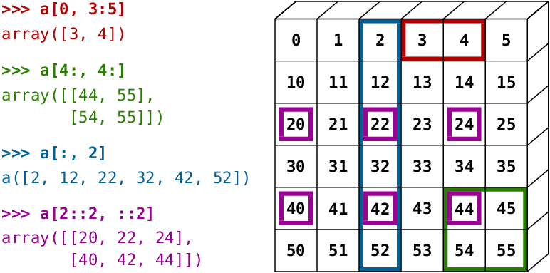
1.5 索引与切片

• 与普通的Python序列一样，NumPy的序列也可以通过索引访问或赋值
• 也可以使用普通Python序列的习惯性用法array[::-1]来使数组逆序
• 在多维数组中，可以通过索引得到一个元组
• 与普通的Python序列一样，NumPy的序列也可以通过array[start:end:step]进行切片。其中，start缺省为0，end缺省为最后一个元素，step缺省为1。
• 注：最后一个索引并不包含的切出的序列之中，如array[:4]仅包含索引为0,1,2,3的元素。
• 也可以一边切片，一边赋值:

a = np.arange(10)
a[5:] = 10
a   # array([ 0,  1,  2,  3,  4, 10, 10, 10, 10, 10])
b = np.arange(5)
a[5:] = b[::-1]
a   # array([0, 1, 2, 3, 4, 4, 3, 2, 1, 0])

1.6 拷贝与视图

A slicing operation creates a view on the original array, which is
just a way of accessing array data. Thus the original array is not
copied in memory. You can use np.may_share_memory() to check if # two
arrays share the same memory block. Note however, that this uses
heuristics and may give you false positives.
切片操作的结果，仅仅是在原数组上产生一个视图，以此达到访问数据的目的。因此，原始数组并没有被拷贝到内存中，可以使用np.may_share_memory()来查看两个数组是否共享内存。注意，这里使用了启发式方法，可能会有误报。

• 当改变视图时，原始数组的数据也会跟着改变

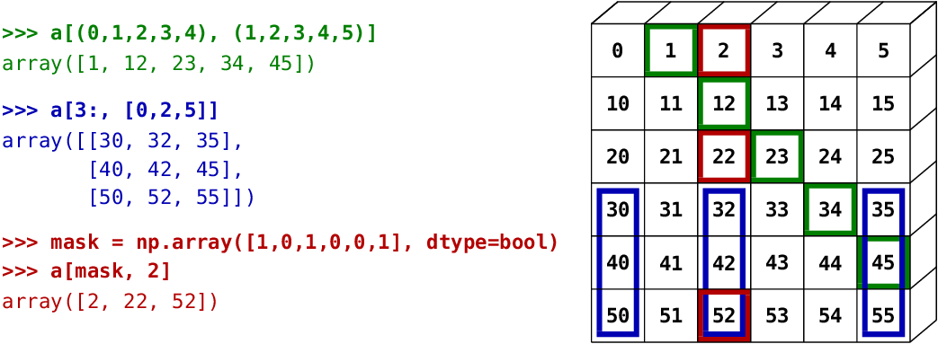
1.7 花式索引 Fancy indexing

NumPy arrays can be indexed with slices, but also with boolean or
integer arrays (masks). This method is called fancy indexing. It
creates copies not views.
NumPy数组可以通过切片索引，也可以使用布尔值或整数数组（掩码）进行索引。这种方法叫做花式索引。 它创建的是副本而非视图。

1.7.1 使用bool掩码

# 通过花式索引，切片得到仅包含3的倍数的新数组
np.random.seed(3)
a = np.random.random_integers(0, 20, 15)
a # array([10,  3,  8,  0, 19, 10, 11,  9, 10,  6,  0, 20, 12,  7, 14])
b = (a % 3 == 0) # 得到一个与a一样长的bool数组。在相同的索引位置i上，若a[i]为3的倍数，则b[i]为True，否则为False
extract_from_a = a[mask] #  array([ 3,  0,  9,  6,  0, 12])
a[a % 3 == 0] = -1       # 3的倍数都被赋值为-1

1.7.2 使用整数数组的花式索引

a = np.arange(0, 100, 10) # 创建一个数组 a
# 索引可以是也一个整数数组，相同的索引可以重复
a[[2, 3, 2, 4, 2]]  # array([20, 30, 20, 40, 20]) 
# 也可以通过以下方式进行赋值
a[[9, 7]] = -100 # array([0,10,20,30,40,50,60,-100,80,-100])
# 当通过整数数组花式索引index创建一个新数组时，新数组与index形状相同
a = np.arange(10)
index = np.array([[3, 4], [9, 7]]) # index.shape = (2, 2)
a[index]    # array([[3, 4],[9, 7]])

2. 数组数值运算 Numerical operations on arrays

2.1 智慧数组操作 Elementwise operations

2.1.1 基本操作

可进行基本的+-*/操作

a = np.array([1, 2, 3, 4])
b = np.ones(4) + 1
a + 1   # 每个元素+1
2**a# 每个元素平方
a - b   # 每个元素相减
a * b   # 每个元素相乘
j = np.arange(5) 
2**(j + 1) - j # 批量操作  
# 数组间的乘法为c.dot(c)

2.1.2 其他操作

数组的比较

a = np.array([1, 2, 3, 4])
b = np.array([4, 2, 2, 4])
a == b
a > b # 逐元素比较，返回一个bool数组

数组整体进行比较

a = np.array([1, 2, 3, 4])
b = np.array([4, 2, 2, 4])
c = np.array([1, 2, 3, 4])
np.array_equal(a, b)
np.array_equal(a, c)  # 整个数组进行比较返回bool值

逻辑操作(Logical operations)

a = np.array([1, 1, 0, 0], dtype=bool) 
b = np.array([1, 0, 1, 0] dtype=bool) 
np.logical_or(a, b) 
np.logical_and(a, b)

超越函数(Transcendental Functions)

指变量之间的关系不能用有限次加、减、乘、除、乘方、开方运算表示的函数。

a = np.arange(5)
np.sin(a)
np.log(a)
np.exp(a)

矩阵逆置(Transposition)

a = np.triu(np.ones((3, 3)), 1)   # 上三角行列式 np.tril下三角行列式
a.T

2.2 数组/矩阵的基础约简 Basic reductions

2.2.1 计算元素之和

数组

x = np.array([1, 2, 3, 4])
np.sum(x)
x.sum() # 均返回数组元素之和

按行/列求和

x = np.array([[1, 1], [2, 2]])
x.sum(axis=0)   # 列求和，1维求和
x[:, 0].sum(), x[:, 1].sum()
x.sum(axis=1)   # 行求和，第2维求和
x[0, :].sum(), x[1, :].sum()

2.2.2 其它约简

极值

x = np.array([1, 3, 2])
x.min()
x.max()
x.argmin()  # 返回最小值索引
x.argmax()  # 返回最大值索引

逻辑运算

np.all([True, True, False]) # False
np.any([True, True, False]) # True

统计运算

x = np.array([1, 2, 3, 1])
y = np.array([[1, 2, 3], [5, 6, 1]])
x.mean() # 均值
np.median(x) # 中位数
np.median(y, axis=-1) # last axis array([ 2.,  5.])
x.std()  # 标准差

2.3 广播 Broadcasting

It’s also possible to do operations on arrays of different sizes if
NumPy can transform these arrays so that they all have the same size:
this conversion is called broadcasting.
若通过Numpy能将不同形状的数组/矩阵转换为相同形状，则这些数组/矩阵之间可以进行运算。

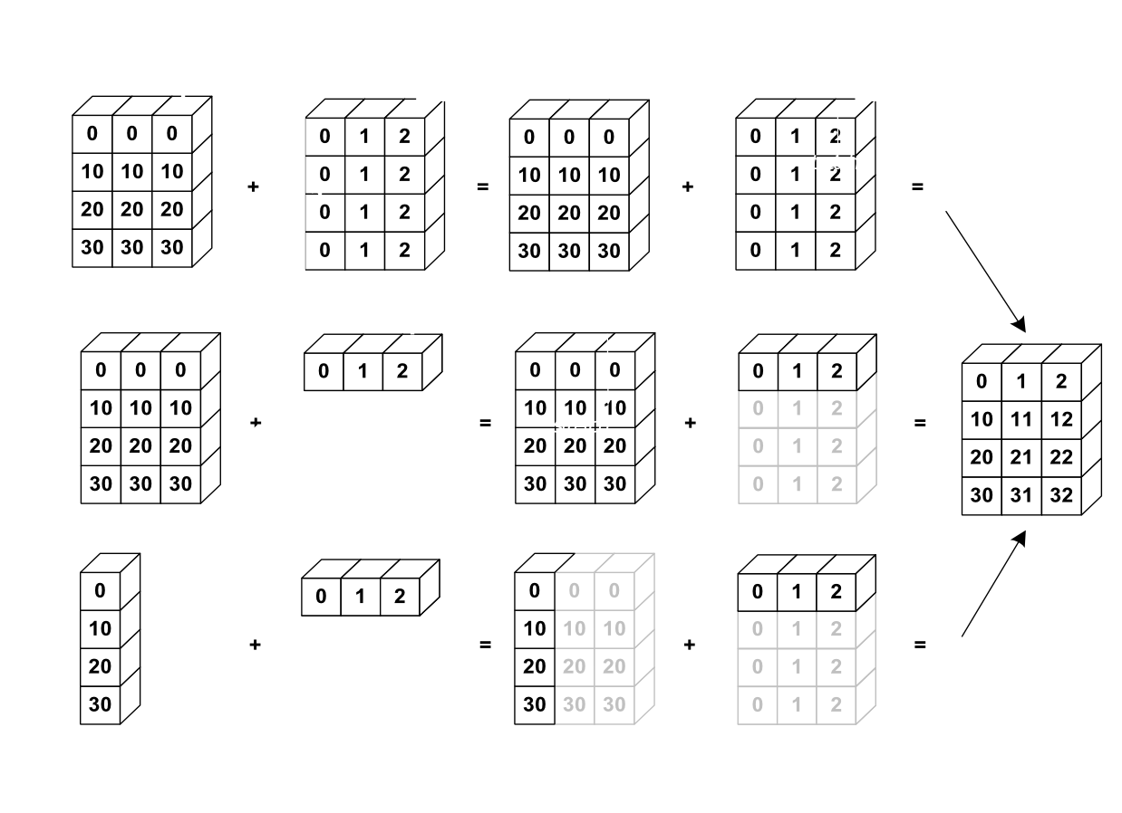
一个常用的技巧

a = np.arange(0, 40, 10)
a.shape
(4,)
a = a[:, np.newaxis]  # adds a new axis -> 2D array
a.shape
(4, 1)
a
array([[ 0],
   [10],
   [20],
   [30]])
a + b
array([[ 0,  1,  2],
   [10, 11, 12],
   [20, 21, 22],
   [30, 31, 32]])

np.ogrid

x, y = np.ogrid[0:5, 0:5]
x, y
(array([[0],
   [1],
   [2],
   [3],
   [4]]), array([[0, 1, 2, 3, 4]]))
x.shape, y.shape
((5, 1), (1, 5))
distance = np.sqrt(x ** 2 + y ** 2)

np.mgrid

x, y = np.mgrid[0:4, 0:4]
x
array([[0, 0, 0, 0],
   [1, 1, 1, 1],
   [2, 2, 2, 2],
   [3, 3, 3, 3]])
y
array([[0, 1, 2, 3],
   [0, 1, 2, 3],
   [0, 1, 2, 3],
   [0, 1, 2, 3]])

2.4 改变数组形状 Array shape manipulation

2.4.1 扁平化 Flattening

np.ravel()

a = np.array([[1, 2, 3], [4, 5, 6]])
a.ravel()
array([1, 2, 3, 4, 5, 6])
a.T
array([[1, 4],
   [2, 5],
   [3, 6]])
a.T.ravel()
array([1, 4, 2, 5, 3, 6])

2.4.2 重塑 Reshaping

Flatting 的逆函数
np.reshape(shape)

2.4.3 升维 Adding a dimension

L = np.arange(0, 3) # shape: (3, )
x = L[:, np.newaxis] # shape: (3, 1)
y = L[np.newaxis, :] # shape: (1, 3)

2.4.4 维度洗牌 Dimension Shuffling

np.transpose() # i与n-i交换维度

2.4.5 重新定义大小 Resizing

np.resize(shape) 注：被resize的数组不能被赋给其他数组

2.5 数据的排序 Sorting data

np.sort(self, asix= )

2.6 总结 Summary

• 创造数组 array,arange,ones,zero
• Know the shape of the array with array.shape, then use slicing to obtain different views of the array: array[::2], etc.
• Adjust the shape of the array using reshape or flatten it with ravel.
• Obtain a subset of the elements of an array and/or modify their values with masks
• Know miscellaneous operations on arrays, such as finding the mean or max (array.max(), array.mean()). No need to retain everything, but have the reflex to search in the documentation (online docs, help(), lookfor())!!
• For advanced use: master the indexing with arrays of integers, as well as broadcasting. Know more NumPy functions to handle various array operations.

3. 更复杂的数组 More elaborate arrays

3.1 更多数据类型 More data types

3.1.1 强制转型 Casting

• 强制转换类型时，“更大的”的类型往往“胜利”

np.array([1, 2, 3]) + 1.5
array([ 2.5,  3.5,  4.5]) # int ---> float

• 赋值不会改变数据类型

a = np.array([1, 2, 3])
a.dtype     # dtype('int64')
a[0] = 1.9  # <-- float is truncated to integer
a           # array([1, 2, 3])

• 强制转型

a = np.array([1.7, 1.2, 1.6])
b = a.astype(int)  # b = array([1, 1, 1]

• 四舍五入

a = np.array([1.2, 1.5, 1.6, 2.5, 3.5, 4.5])
b = np.around(a) # array([ 1.,  2.,  2.,  2.,  4.,  4.])

3.1.2 不同数据类型的大小 Different data type sizes

# 在进行数据运算时，越小的数据类型，速度越快；其所占的空间的要求的宽度也越小
int8/uint8               # 8 bits
int16/uint16/float16     # 16 bits
int32/uint32/float32     # 32 bits
int64/uint64/float64     # 64 bits
float128                 # 128 bits, 取决于平台
complex64   # two 32-bit floats
complex128  # two 64-bit floats
complex192  # two 96-bit floats, 取决于平台
complex256  # two 128-bit floats, 取决于平台

3.2 结构化数据类型 Structured data types

• 支持通过索引访问
• 支持多索引
• 支持花式索引

# 示例 
# sensor_code (4-character string)
# position  (float)
# value (float)
samples = np.zeros((6,), dtype=[('sensor_code', 'S4'), ('position', float), ('value', float)])
samples.ndim        # 1
samples.shape       # (6,)
samples.dtype.names # ('sensor_code', 'position', 'value')

3.3 maskedarray:处理丢失的数据

• For floats one could use NaN’s, but masks work for all types:

x = np.ma.array([1, 2, 3, 4], mask=[0, 1, 0, 1])
x
masked_array(data = [1 -- 3 --],
             mask = [False  True False  True],
       fill_value = 999999)
y = np.ma.array([1, 2, 3, 4], mask=[0, 1, 1, 1])
x + y
masked_array(data = [2 -- -- --],
             mask = [False  True  True  True],
       fill_value = 999999)

• Masking versions of common functions:

np.ma.sqrt([1, -1, 2, -2]) 
masked_array(data = [1.0 -- 1.41421356237... --],
             mask = [False  True False  True],
       fill_value = 1e+20)

4. 高级运算

4.1 多项式 Polynomials

• NumPy支持不同次数的多项式
  e.g. $y = 3x^2 + 2x -1$

p = np.poly1d([3, 2, -1]) 
p(0)        # -1, x=0时y的值
p.roots     # array([-1.,  0.33333333])，顶点
p.order     # 2, 次数

4.1.1 更多的多项式(更高次数) More polynomials (with more bases)

4.2 载入数据文件

4.2.1 文本文件

• 载入文件 np.load('path')
• 保存文件 np.savetxt('path', array)

4.2.2 图片

• 使用Matplotlib包

img = plt.imread('data/elephant.png')
img.shape, img.dtype    # ((200, 300, 3), dtype('float32'))
plt.imshow(img)     
<matplotlib.image.AxesImage object at ...>
plt.savefig('plot.png')
plt.imsave('red_elephant', img[:,:,0], cmap=plt.cm.gray)

4.2.3 NumPy的自有格式

• NumPy有自己的二进制格式，不可移植，但在进行写入/写出操作时比较高效

data = np.ones((3, 3))
np.save('pop.npy', data)
data3 = np.load('pop.npy')

4.2.4 知名的文件格式

• HDF5: h5py, PyTables
• NetCDF: scipy.io.netcdf_file, netcdf4-python, ...
• Matlab: scipy.io.loadmat, scipy.io.savemat
• MatrixMarket: scipy.io.mmread, scipy.io.mmwrite
• IDL: scipy.io.readsav

心血来潮，自娱自乐，供自己参考=.=
mr.yxj@foxmail.com