基于BP神经网络与TF-IDF的文本分类模型

作者：郭渊博 刘越 牛哲

摘要

文本分类主要包括两个阶段：

1. 文本预处理，文本特征提取阶段。
2. 分类阶段。

我们的模型在文本特征提取阶段主要采用了TF-IDF作为文本特征，在分类阶段采用了BP神经网络。

特征提取

1. TF-IDF特征提取

TF-IDF模型的主要思想

如果一个词w在一篇文档d中出现的频率高，且少在其他文档中出现，则认为w有很好的区分能力。

在代码中具体采用了如下公式：

$$T_{tf{-}idf} = T_f*\log(\frac{N}{D_f})$$

其中$T_f$为该词在该篇文章中出现的次数，$N$为总文章数，$D_f$为所有文章中含有该词的文章数。

$\log(\frac{N}{D_f})$值也被称作IDF值，它的大小体现出一个词语的区分能力。

可见，当$D_f$接近于$N$时，也就是当该词几乎被所有文章涵盖，该词的区分能力就很差，此时$\log(\frac{N}{D_f})$的值就为0，而当$D_f$与$N$相差较多时，该词的区分能力就较好，$\log(\frac{N}{D_f})$的值就较大。

TF-IDF模型的具体使用

首先取出所有词语（所有文档词语的并集）中词频最高的300词作为提取特征的基础：

self.top_freq_word = self.freq_dist.most_common(300)

在这300词中，统计每个词在所有文章中出现的次数：

for word, freq in self.top_freq_word:
    for x, y in self.train_set:
        if word in x:
            if self.df.has_key(word):
                self.df[word] += 1
            else:
                self.df[word] = 1

最后，对每个词计算 $T_{tf{-}idf}$，并将结果加到特征集中：

for word, freq in self.top_freq_word:
    features.append(doc.count(word)*math.log(len(self.train_set)/self.df[word]))

2. 罕见词语计数特征提取

罕见词语计数的主要思想

由于一些罕见词语只出现在单独的一种文档之中，故在对训练文档进行预处理时，提取出那些只出现在一种文档中的词语，并对其进行标记。之后，对于每个不同文档类型，统计一篇文档所拥有的该类型的罕见词语数量，并将这些类型-罕见词语数量对应关系作为特征。

罕见词语计数的具体使用

初始化

#每个类型文章所包含的所有词语
self.labeled_words = {}
for x, y in self.train_set:
    idx = self.label_set.index(y)
    if self.labeled_words.has_key(idx):
        self.labeled_words[idx] |= set(x)
    else:
        self.labeled_words[idx] = set(x)
#每个类型文章所包含的所有罕见词语
self.labeled_words_clean = {}
#先赋值为每个类型文章包含的所有词语
for k in self.labeled_words:
    self.labeled_words_clean[k] = set(self.labeled_words[k])
#接下来对每一个类型文章的词语集合与其它类型文章的词语集合进行差运算
#以算出每个类型文章的罕见词语集合
for k1 in self.labeled_words_clean:
    for k2 in self.labeled_words:
        if k1 != k2:
                self.labeled_words_clean[k1] -= self.labeled_words[k2]

特征化

#对于每种类型文档的所有罕见词语，统计该篇文章所包含的该类型的罕见词语数量
for k in self.labeled_words_clean:
    cnt = 0
    for word in doc:
        if word in self.labeled_words_clean[k]:
            cnt += 1
    features.append(cnt)

分类

BP神经网络简介

神经元

神经元是神经网络的基本单元，它的结构如下图所示：

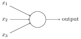
在神经元中，每一个输入边上都有一个边权，记为$w_j$，每个神经元有一个偏值(bias)，记为$b$，在所有输入信号输入之后，便可得到神经元计算加权的输入$z$：

$$z=\sum_j w_j x_j + b\tag{1}$$
加权输入$z$经过一个激活函数(activation function)$\sigma$，得到该神经元的输出$a$：
$$a=\sigma(z)\tag{2}$$

常用的激活函数有：

1. Step函数
   $$\begin{eqnarray} \sigma(z) = \left\{ \begin{array}{ll} 0 & z \leq 0 \\\\ 1 & z > 0 \end{array} \right. \tag{3}\end{eqnarray}$$
2. Sigmoid函数
   $$\begin{eqnarray} \sigma(z) = \frac{1}{1+e^{-z}}. \tag{4}\end{eqnarray}$$
3. Tanh函数
   $$\begin{eqnarray} \sigma(z) = tanh(z). \tag{5}\end{eqnarray}$$

等，我们的模型采用Sigmoid激活函数

对与某个输入$x$，得到输出$a$为预测结果，实际结果$y(x)$,通过计算开销$Cost$：

$$\begin{eqnarray} C(w,b) \equiv \frac{1}{2n} \sum_x \| y(x) - a\|^2. \tag{6}\end{eqnarray}$$

其中$w, b$为该神经元的权重和偏值，$y(x)$为实际的结果，$a$为神经元输出的结果，$n$为训练的样本总数。我们希望$C(w,b)$越小越好。

前向神经网络

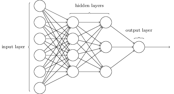
多个神经元构成神经网络的一层，从而构成一个神经网络。神经网络的第一层与最后一层被称为输入层和输出层，中间的层被称为隐含层。输入层的神经元个数与输入特征的维数相同，输出层神经元的个数与分类的类别数相同。隐含层的层数与每层神经元个数根据具体的模型进行调节，通过调节隐含层的层数与每层神经元个数可以避免欠拟合与过拟合。在前向神经网络中，每一个前一层的神经元的输出都跟下一层的神经元相连。

将多个神经元连接起来之后，整个神经网络的$Cost$函数如下：

$$\begin{eqnarray} C(w,b) \equiv \frac{1}{2n} \sum_x \| y(x) - a\|^2. \tag{7}\end{eqnarray}$$

其中$y(x)$为一个以神经网络输出层神经元数为维数的向量，$a$为神经网络最后一层的输出向量，对于每一个输入向量$x$（即每一个训练数据）我们希望通过调节参数$w, b$使得$Cost$函数的最终值最小。

我们通过Back Propagation的方法，将这个差值的影响从输出层一层一层地向后传，从而将神经网络的所有层进行调参。

Back Propagation

（公式不在此篇文章中证明，若需了解证明过程，请参考^[1])

其中$\odot$符号的含义是指对两个维数相同的向量，将其对应的每一项相乘，例如：

$$\begin{eqnarray} \left[\begin{array}{c} 1 \\ 2 \end{array}\right] \odot \left[\begin{array}{c} 3 \\ 4\end{array} \right] = \left[ \begin{array}{c} 1 * 3 \\ 2 * 4 \end{array} \right] = \left[ \begin{array}{c} 3 \\ 8 \end{array} \right]. \tag{8}\end{eqnarray}$$

对于最后一层（L层），式子BP1计算出了中间量$\delta^L$，BP2则使得中间量$\delta^l$一层一层地向后传播，BP3给出了$Cost$根据$b^l_j$（第l层第j个神经元的偏值）的偏导$\frac{\partial C}{\partial b^l_j}$，值为$\delta^l_j$，BP4给出了$Cost$根据权值跟$w^l_{jk}$（第l层第j个神经元跟前一层第k个神经元之间连线的权重）的偏导$\frac {\partial C}{\partial w^l_{jk}}$，值为$a^{l-1}_k\delta^l_j$。

由于沿着梯度方向$Cost$函数下降最快，所以每次训练后经过Back Propagation得到的$\frac{\partial C}{\partial b^l_j}$与$\frac {\partial C}{\partial w^l_{jk}}$正是相应变量需要改变的值，根据以下方式对变量进行更新：

$$b^l_j \leftarrow b^l_j + eta\cdot\frac{\partial C}{\partial b^l_j} \tag{9}$$
$$w^l_{jk} \leftarrow w^l_{jk} + eta\cdot\frac {\partial C}{\partial w^l_{jk}} \tag{10}$$

其中$eta$为学习速率，$eta$值越小，收敛越慢，但更精确。

在不断调整$w, b$后，我们便可得到较小的$Cost$值。

BP神经网络的具体使用

import numpy as np
import random 
def sigmoid(z):
    return 1.0/(1.0+np.exp(-z))
def sigmoid_prime(z):
    return sigmoid(z)*(1-sigmoid(z))
class Network(object):
    def __init__(self, layers):
        self.layers = layers
        self.weights = [np.random.randn(x, y) for x, y in zip(layers[:-1], layers[1:])]
        self.biases = [np.random.randn(1, y) for y in layers[1:]]
    def feedforward(self, activation):
        for weight, bias in zip(self.weights, self.biases):
            activation = sigmoid(np.dot(activation, weight)+bias)
        return activation
    def vectorized_result(self, y):
        e = np.zeros((1, self.layers[-1]))
        e[0][y] = 1.0
        return e
    def train(self, epochs, eta, batch_size, training_data, test_data=None):
        training_data = [(np.reshape(x, (1, len(x))), self.vectorized_result(y)) for x, y in training_data]
        test_data = [(np.reshape(x, (1, len(x))), y) for x, y in test_data]
        training_data_size = len(training_data)
        if test_data:
            test_data_size = len(test_data)
        for i in xrange(0, epochs):
            random.shuffle(training_data)
            #计算batch，由于我们的batch_size为1，所以一个训练数据为一个batch
            batches = [training_data[k:k+batch_size] for k in xrange(0, training_data_size, batch_size)]
            for batch in batches:
                #更新神经网络
                self.update(batch, eta)
            if test_data:
                #模型测试
                p1 = self.evaluate(test_data)
                p2 = test_data_size
                print "Epoch {0}: {1} / {2} = {3}".format(i, p1, p2, p1*1.0/p2)
            else:
                print "Epoch {0} complete".format(i)
    def update(self, batch, eta):
        batch_size = len(batch)
        nabla_weights = [np.zeros(w.shape) for w in self.weights]
        nabla_biases = [np.zeros(b.shape) for b in self.biases]
        #这里是同时计算多个训练数据的Cost关于w, b的偏导值， 由于我们的batch大小为1，所以nw(nb)与dnw(dnb)相同
        #若batch大小为其他值，则nw(nb)是这些dnw(dnb)的平均值
        for x, y in batch:
            delta_nabla_weights, delta_nabla_biases = self.backprop(x, y)
            nabla_weights = [nw+dnw for nw, dnw in zip(nabla_weights, delta_nabla_weights)]
            nabla_biases = [nb+dnb for nb, dnb in zip(nabla_biases, delta_nabla_biases)]
        #在这里更新w, b
        self.weights = [w-(eta/batch_size)*nw for w, nw in zip(self.weights, nabla_weights)]
        self.biases = [b-(eta/batch_size)*nb for b, nb in zip(self.biases, nabla_biases)]
    #进行back propagation计算
    def backprop(self, x, y):
        activation = x
        activations = [x]
        zs = []
        #一次正向传播算出预测的a值
        for weight, bias in zip(self.weights, self.biases):
            z = np.dot(activation, weight)+bias
            zs.append(z)
            activation = sigmoid(z)
            activations.append(activation)
        #算出最后一层的delta
        delta = (activation-y)*sigmoid_prime(zs[-1])
        #初始化Cost关于w, b的偏导
        nabla_weights = [np.zeros(w.shape) for w in self.weights]
        nabla_biases = [np.zeros(b.shape) for b in self.biases]
        nabla_weights[-1] = np.dot(activations[-2].transpose(), delta)
        nabla_biases[-1] = delta
        #反向计算每一层的delta，并且算出Cost关于w, b的偏导值
        for l in xrange(2, len(self.layers)):
            delta = np.dot(delta, self.weights[-l+1].transpose())*sigmoid_prime(zs[-l])
            nabla_weights[-l] = np.dot(activations[-l-1].transpose(), delta)
            nabla_biases[-l] = delta
        return (nabla_weights, nabla_biases)
    def evaluate(self, test_data):
        result = [(np.argmax(self.feedforward(x)), y) for (x, y) in test_data]
        return sum(int(x==y) for x, y in result)

在backprop函数中，根据一个训练数据，计算出相应的$\frac{\partial C}{\partial b}, \frac{\partial C}{\partial w}$的值，进入update函数对$w, b$进行更新，以完成一次训练。

在evaluate函数中使用测试数据对模型进行评估，feedforward函数算出测试集数据的$a$向量，选出向量中数值最大的相应维度为预测结果，与测试集数据的$y$进行对比，以此来进行评估统计。

输入的训练集的标签，也就是$y$值需要先进行向量化，以满足后面计算的需要。方式即在$y$值所对应的维度将值设置为1，其余值设置为0。

结果分析

运行结果

附录A文件

this is the output of main.py processing data set A
features: only tf-idf
features dimension: 300
network parameter: epoch: 20, learning rate: 1.0, layers: [300, 50, 8]
Epoch 0: 1777 / 2009 = 0.884519661523
Epoch 1: 1842 / 2009 = 0.9168740667
Epoch 2: 1870 / 2009 = 0.93081134893
Epoch 3: 1879 / 2009 = 0.935291189647
Epoch 4: 1902 / 2009 = 0.946739671478
Epoch 5: 1894 / 2009 = 0.942757590841
Epoch 6: 1870 / 2009 = 0.93081134893
Epoch 7: 1898 / 2009 = 0.94474863116
Epoch 8: 1892 / 2009 = 0.941762070682
Epoch 9: 1917 / 2009 = 0.954206072673
Epoch 10: 1915 / 2009 = 0.953210552514
Epoch 11: 1922 / 2009 = 0.956694873071
Epoch 12: 1915 / 2009 = 0.953210552514
Epoch 13: 1915 / 2009 = 0.953210552514
Epoch 14: 1901 / 2009 = 0.946241911399
Epoch 15: 1925 / 2009 = 0.95818815331
Epoch 16: 1909 / 2009 = 0.950223992036
Epoch 17: 1913 / 2009 = 0.952215032354
Epoch 18: 1919 / 2009 = 0.955201592832
Epoch 19: 1922 / 2009 = 0.956694873071
cost time(exclude preprocess time): 19.9823410511 seconds

附录B文件

this is the output of main.py processing data set B
features: tf-idf with rare word count
features dimension: 320
network parameter: epoch: 20, learning rate: 1.0, layers: [320, 50, 20]
Epoch 0: 2084 / 5645 = 0.369176262179
Epoch 1: 3164 / 5645 = 0.560496014172
Epoch 2: 3324 / 5645 = 0.588839681134
Epoch 3: 3378 / 5645 = 0.598405668733
Epoch 4: 3575 / 5645 = 0.63330380868
Epoch 5: 3572 / 5645 = 0.632772364925
Epoch 6: 3634 / 5645 = 0.643755535872
Epoch 7: 3629 / 5645 = 0.64286979628
Epoch 8: 3599 / 5645 = 0.637555358725
Epoch 9: 3659 / 5645 = 0.648184233835
Epoch 10: 3675 / 5645 = 0.651018600531
Epoch 11: 3686 / 5645 = 0.652967227635
Epoch 12: 3689 / 5645 = 0.653498671391
Epoch 13: 3685 / 5645 = 0.652790079717
Epoch 14: 3692 / 5645 = 0.654030115146
Epoch 15: 3693 / 5645 = 0.654207263065
Epoch 16: 3729 / 5645 = 0.660584588131
Epoch 17: 3688 / 5645 = 0.653321523472
Epoch 18: 3681 / 5645 = 0.652081488043
Epoch 19: 3698 / 5645 = 0.655093002657
cost time(exclude preprocess time): 26.7541799545 seconds

附录C文件

this is the output of mainzh.py processing data set C
features: tf-idf with rare word count
features dimension: 308
network parameter: epoch: 20, learning rate: 1.0, layers: [308, 50, 8]
Epoch 0: 58 / 80 = 0.725
Epoch 1: 66 / 80 = 0.825
Epoch 2: 70 / 80 = 0.875
Epoch 3: 71 / 80 = 0.8875
Epoch 4: 71 / 80 = 0.8875
Epoch 5: 71 / 80 = 0.8875
Epoch 6: 70 / 80 = 0.875
Epoch 7: 71 / 80 = 0.8875
Epoch 8: 71 / 80 = 0.8875
Epoch 9: 71 / 80 = 0.8875
Epoch 10: 70 / 80 = 0.875
Epoch 11: 70 / 80 = 0.875
Epoch 12: 72 / 80 = 0.9
Epoch 13: 72 / 80 = 0.9
Epoch 14: 72 / 80 = 0.9
Epoch 15: 72 / 80 = 0.9
Epoch 16: 72 / 80 = 0.9
Epoch 17: 72 / 80 = 0.9
Epoch 18: 72 / 80 = 0.9
Epoch 19: 72 / 80 = 0.9
cost time(exclude preprocess time): 9.03512907028 seconds

结果分析

对于三个附录文件，分类的训练次数皆为20次，最终结果为：

数据集	准确率	用时/秒
附录A	95.67%	19.98
附录B	65.51%	26.75
附录C	90.00%	9.04

可见，该模型对附录A数据和附录C数据的分类效果较好，对附录B数据的分类效果欠佳，我们正在寻找原因，并努力改进。

参考文献

[1]Michael A. Nielsen. "Neural Networks and Deep Learning", Determination Press, 2015
[2]Steven Bird, Ewan Klein, Edward Loper. "Natural Language Processing with Python", O'Reilly Media, 2009.
[3]周志华.机器学习,清华大学出版社,2016.